Principles and Applications of Modern
DNA Sequencing
EEEB GU4055
Session 4: Scientific Python
Today's topics
1. review of topics thus far.
2. file I/O
3. fastq to fasta
4. genome annotation
5. introducing numpy and pandas
Python Dictionaries
A look-up table. Store values associated with look-up keys. Very efficient data structure for storing and retrieving data.
  # make a dict using curly bracket format
  adict = {
    'key1': 'val1',
    'key2': 'val2',
  }

  # request a value using a key
  print(adict['key1'])
val1
Comments are a key part of writing good code
  # import the random library
  import random

  # create a list with 1000 random numbers between 0-10
  integer_list = [random.randint(0, 10) for i in range(1000)]

  # create an empty dictionary
  counter = {}

  # iterate over elements of the integer list
  for item in integer_list:

      # conditional True if item is not already in the dict keys
      if item not in counter:
          # set the value to 1 for this key
          counter[item] = 1

      # item is already in dict keys
      else:
          # increment value by 1 for this key
          counter[item] += 1
Python Advanced
You have now learned all of the core object types in Python. From these simple objects more complex Python object can be built. Thousands of complex software tools have been developed from creatively combining these objects with Python coding routines.
  # The core Python object types
  a_integer = 8
  b_float = 0.2345
  c_string = "a string"
  d_list = ["a", "list", "of", "strings"]
  e_tuple = ("a", "tuple", "of", "strings")
  f_dict = {"a key": ["and value in a dictionary"]}
File I/O: bash to Python
  %%bash
  wget http://eaton-lab.org/data/40578.fastq.gz -q -O 40578.fastq.gz
  import os
  import gzip
  import requests

  # the URL to file 1
  url1 = "https://eaton-lab.org/data/40578.fastq.gz"

  # open a file for writing and write the content to it
  with gzip.open("40578.fastq.gz", 'wb') as ffile:
      ffile.write(requests.get(url1).content)
File I/O: file objects
Reading and writing files in Python is done through File objects. You first create an object, then use it is some way (functions), and finally close it.
  # open a file object in write-mode
  ofile = open("./datafiles/helloworld.txt", 'w')

  # write a string to the file
  ofile.write("hello world")

  # close the file object
  ofile.close()
File I/O: file objects
The term 'with' creates context-dependence within the indented block. The object can have functions that are automatically called when the block starts or ends. For an open file object the block ending calls .close(). This often is simpler better code.
  # a simpler alternative: use 'with', 'as', and indentation
  with open("./helloworld.txt", 'w') as ofile:
      ofile.write("hello world")
File I/O: file objects
To reiterate, these two code blocks are equivalent.
  # open a file object in write-mode
  ofile = open("./helloworld.txt", 'w')

  # write a string to the file
  ofile.write("hello world")

  # close the file object
  ofile.close()
  # a simpler alternative: use 'with', 'as', and indentation
  with open("./helloworld.txt", 'w') as ofile:
      ofile.write("hello world")
File I/O: file objects
Compression or decompression is as simple as writing or reading using a File object from a compression library (e.g., gzip or bz2).
  import gzip

  # open a gzipped file object in write-mode to expect byte strings
  ofile = gzip.open("./helloworld.txt", 'wb')

  # write a byte-string to the file
  ofile.write(b"hello world")

  # close the file object
  ofile.close()
File I/O: reading
Open a file and call .read() to load all of the contents at once to a string or bytes object.
  # open a file
  fobj = open("./data.txt", 'r')

  # read data from this file to create a string object
  fdata = fobj.read()

  # close the file
  fobj.close()

  # print part of the string 'fdata'
  print(fdata[:500])
File I/O: reading
Open a file and call .read() to load all of the contents at once to a string or bytes object.
  # open a gzip file
  fobj = gzip.open("./data.fastq", 'r')

  # read compressed data from this file and decode it
  fdata = fobj.read().decode()

  # close the file
  fobj.close()

  # print part of the string 'fdata'
  print(fdata[:500])
File I/O: reading
Once again, the 'with' context style of code is a bit more concise.
  # open a gzip file and read data using 'with'
  with gzip.open("./data.fastq", 'r') as fobj:
      fdata = fobj.read().decode()
      print(fdata[:500])
File I/O: file paths
File paths are an important concept to master in bioinformatics. Be aware of the absolute path to where you are, and where the files you want to operate on are located, and understand how relative paths can also point to these locations.
  # os.path.abspath() prints the absolute path from a relative path
  os.path.abspath(".")

  # os.path.join() combines two or more parts of paths together with /
  os.path.join("/home/deren", "file1.txt")

  # os.path.basename() and os.path.dirname() return the dir and filename
  os.path.basename("/home/deren/file.txt")

  # check if a file exists before trying to do something with it
  os.path.exists("badfilename.txt")
The FASTA file format
The fasta format is commonly used to store sequence data. We learned about it in our first notebook assignment and also saw some empirical examples representing full genomes. The delimiter ">" separates sequences. Files typically end in .fasta, .fna, (DNA specific) or .faa (amino acids specific).
  >mus musculus gene A
  AGTCAGTCAGCGCTAGTCATAACACGCAAGTCAATATATACGACAGCAGCTAGCTACTTCGACA
  CAGTCGATCAGCTAGCTGACTACTATATATTTTTATATGTAAAAAAAACATATGCGCGCTTTTG
  GGGGAGTATTTTATGCATATCATGCAGCATATAGGTAGCTGTGCATGCTGCTAGCACGATCGTA
  CATGCTAGCTAGCTAGCTAGCTAGCTAGCTGACTAGCTAGTGCTAGCTAGCTATATATATATAT

  >mus musculus gene B
  ACGTACGTACGTACGTAGCTAGCTACATGCTAGCATGCATGCTAGCTAGCTATATATAGCCCCC
  CAGCGGGGGGCGTCATGCATAAAAAAAAAAAGCATCATGCCGCGCCCCTAGCGCGTATTTTCTT
  ...
The FASTA file format
Challenge: Write code to combine a fasta header (e.g., "> sequence name") and a random sequence of DNA to a create valid fasta data string. Then write the data to a file and save it as "datafiles/sequence.fasta".
  # a function to return a random DNA string
  def random_dna(length):
      dna = "".join([random.choice("ACGT") for i in range(length)])
      return dna

  # format dna string to fasta format
  dna = random_dna(20)
  fasta = "> sequence name\n" + dna

  # write it to a file
  with open("./datafiles/sequence.fasta", 'w') as out:
      out.write(fasta)
The FASTQ file format
The fastq format is commonly used to store sequenced read data. It differs from fasta in that it contains quality (confidence) scores. Each sequenced read represented by four lines, and a single file can contain many millions of reads.
  @SEQ_ID
  GATTTGGGGTTCAAAGCAGTATCGATCAAATAGTAAATCCATTTGTTCAACTCACAGTTT
  +
  !''*((((***+))%%%++)(%%%%).1***-+*''))**55CCF>>>>>>CCCCCCC65
FASTQ quality scores
Quality scores are encoded using ASCII characters, where each
character can be translated into an integer score that is
log10 probability the base call is incorrect:
$$ Q = -10 * log_{10}(P) $$
  # load a phred Q score as a string:
  phred = "IIIIIGHIIIIIHIIIIFIIIDIHGIIIBGIIFIDIDI"

  # ord() translates ascii to numeric
  q_scores = [ord(i) for i in phred]

  # values are offset by 33 on modern Illumina machines
  q_scores = [ord(i) - 33 for i in phred]
  print(q_scores)
[40, 40, 40, 40, 40, 38, 39, 40, 40, 40, 40, 40, 39, 40, 40, ...
FASTQ quality scores
Quality score is an integer log10 probability the base call
is incorrect:
$$ Q = -10 * log_{10}(P) $$
  # Q=30 means 3 decimal places in the probability of being wrong (0.001)
  import math
  print(-10 * math.log10(0.001))

  # print the probability associated with the first few q_scores
  probs = [10 ** (q / -10) for q in q_scores]
  print(probs)
  30.0
  [0.0001, 0.0001, 0.0001, 0.0001, 0.0001, 0.00015848931924611142, ...
FASTQ conversion
Now that you understand reading and writing files, working with string and list objects, and the format of fastq and fasta file formats, you are prepared to write a function to convert from one to the other.
  def fastq2fasta(in_fastq, out_fasta):
      """
      (1) Write a function;
      (2) read 'datafiles/40578.fastq.gz' from disk;
      (3) convert to fasta format; and
      (4) write result to a file
      """
      # 2. read in the fastq file
      with gzip.open(in_fastq, 'rb') as indata:
          fastq = indata.read().decode()

      # 3. convert to fasta: start with an empty list
      fastadata = []

      # split file into separate reads on \n@ delimiter
      reads = fastq.split("\n@")
      for read in reads:
          # split read into 4 lines
          lines = read.split("\n")

          # join ">", line[0], and line[1] to make fasta formatted sequence
          fastadata.append(">" + lines[0] + "\n" + lines[1])

      # join strings in the list back together into a string
      fasta = "\n".join(fastadata)

      # write to a file
      with open(out_fasta, 'w') as out:
          out.write(fasta)
Dictionaries in action: translation
  GENCODE = {
      'ATA': 'I', 'ATC': 'I', 'ATT': 'I', 'ATG': 'M',
      'ACA': 'T', 'ACC': 'T', 'ACG': 'T', 'ACT': 'T',
      'AAC': 'N', 'AAT': 'N', 'AAA': 'K', 'AAG': 'K',
      'AGC': 'S', 'AGT': 'S', 'AGA': 'R', 'AGG': 'R',
      'CTA': 'L', 'CTC': 'L', 'CTG': 'L', 'CTT': 'L',
      'CCA': 'P', 'CCC': 'P', 'CCG': 'P', 'CCT': 'P',
      'CAC': 'H', 'CAT': 'H', 'CAA': 'Q', 'CAG': 'Q',
      'CGA': 'R', 'CGC': 'R', 'CGG': 'R', 'CGT': 'R',
      'GTA': 'V', 'GTC': 'V', 'GTG': 'V', 'GTT': 'V',
      'GCA': 'A', 'GCC': 'A', 'GCG': 'A', 'GCT': 'A',
      'GAC': 'D', 'GAT': 'D', 'GAA': 'E', 'GAG': 'E',
      'GGA': 'G', 'GGC': 'G', 'GGG': 'G', 'GGT': 'G',
      'TCA': 'S', 'TCC': 'S', 'TCG': 'S', 'TCT': 'S',
      'TTC': 'F', 'TTT': 'F', 'TTA': 'L', 'TTG': 'L',
      'TAC': 'Y', 'TAT': 'Y', 'TAA': '_', 'TAG': '_',
      'TGC': 'C', 'TGT': 'C', 'TGA': '_', 'TGG': 'W',
  }
  GENCODE["CTA"]
L
How are genes identified?
Genome annotation is the process of labeling genomic elements,
including genes and their parts. Your reading by Yandell and Ence
introduces the concepts of genome annotation, a process that
has evolved rapidly over the last decade.
We used a translation dictionary in Python to search a string
of DNA for start and stop codons to an open reading frame (ORF)
: a region that could be translated. This was a relatively crude approach.
Modern approaches use RNA-seq, in which RNA is extracted and reverse-transcribed into cDNA
-- the subset of the genome matching to coding genes -- that
is then sequenced and mapped to a reference genome. Thus we only
examine a subset of the genome for annotation.
Genome annotations in practice
Annotated genomes of model organisms, like humans and
Drosophila, are works in progress. However, they are considered
to be highly accurate in comparison to most other genomes that
have been sequenced recently. This is because their genomes are
assembled better (more contiguous), and because they are able to
build upon decades of experimental work to infer the function
of genes.
Your next assignment will cover assembly statistics, like N50,
what it means, how to calculate it, and what type of values
represent good versus poor genome assemblies.
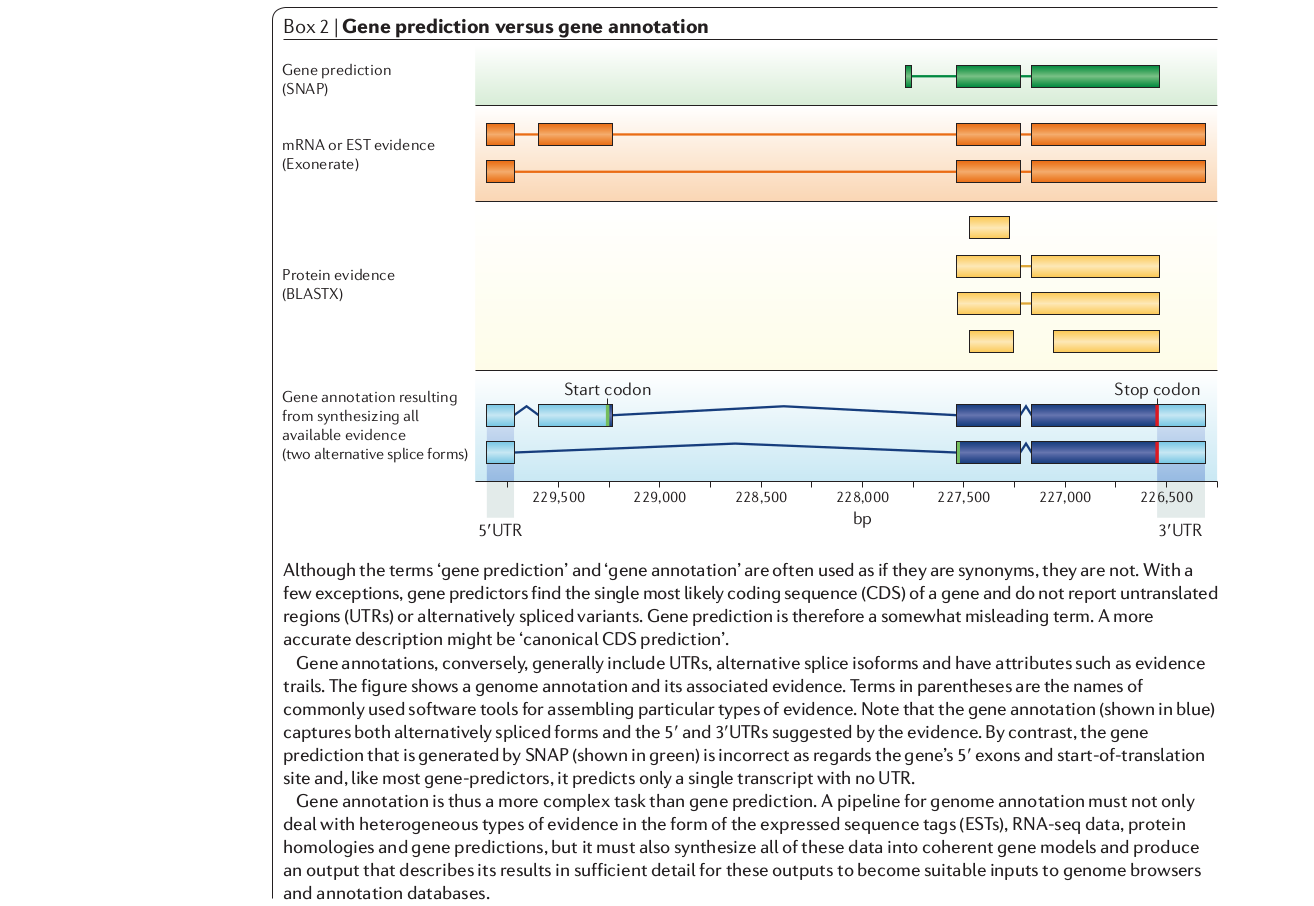
Genome annotations in practice
1. Repeat mask the genome to prevent data mapping to
repetitive regions (e.g., transposons), which also have
open reading frames (ORFs) and can interfere with the
identification of other ORFs associated with genes.
2. Map RNA-seq reads to a reference (e.g., using TopHat) and assemble
transcript contigs from overlapping mapped reads (e.g., using
Cufflinks).
3. ab initio gene prediction: little or no external evidence. Find the most likely coding sequence (CDS) in ORFs. Model parameters (e.g., GC content, intron lengths) affect accuracy, and vary among organisms. Additional evidence includes RNA-seq and Protein sequence data to identify introns/exons and UTRs.
4. Annotation: combining evidence from multiple data types or analyses.
Two more Python object: Arrays and DataFrames
numpy and pandas are the reason Python is popular for data science.
  # numpy arrays are similar to lists, but also very different.
  import numpy as np
  arr = np.array([0, 5, 2, 1, 14])

  # pandas dataframes are tables {column name: data}
  import pandas as pd
  df = pd.DataFrame({"column1": arr})
  [ 0  5  2  1 14]
     column1
  0        0
  1        5
  2        2
  3        1
  4       14
A short numpy intro
numpy arrays are super efficient data structures. All data in an array is of the same type (int8, int64, float64) which makes computations fast. In addition, is performs broadcasting on arrays and includes many numerical functions.
  # create an array from a list
  arr = np.array([0, 5, 2, 1, 14])

  # create a 1-d array of all zeros
  arr = np.zeros(100)

  # create a 2-d array of all zeros
  arr = np.zeros((10, 10))

  # create a 2-d array of all zeros of integer type data
  arr = np.zeros((10, 10), dtype=np.int8)
A short numpy intro
numpy arrays are super fast and efficient. All data is of the same 'type' (int8, int64, float64). Functions can be 'broadcast', and many numerical functions are supported.
  # array of 1-10 reshaped to be 5 rows 2 columns
  narr = np.arange(10).reshape((5, 2))
  # print the shape of the array
  print(narr.shape)
  # arrays can be indexed just like lists
  print(narr)
  (5, 2)
  array([[0, 1],
         [2, 3],
         [4, 5],
         [6, 7],
         [8, 9]])
A short numpy intro
numpy arrays are super fast and efficient. All data is of the same 'type' (int8, int64, float64). Functions can be 'broadcast', and many numerical functions are supported.
  # two arrays can be added together value-by-value
  xarr = np.arange(10) + np.arange(10)

  # to lists are concatenated when added, not processed per-value
  larr = list(range(10)) + list(range(10))

  print(xarr)
  print(larr)
[ 0  2  4  6  8 10 12 14 16 18]
[0, 1, 2, 3, 4, 5, 6, 7, 8, 9, 0, 1, 2, 3, 4, 5, 6, 7, 8, 9]
A short numpy intro
numpy arrays are super fast and efficient. All data is of the same 'type' (int8, int64, float64). Functions can be 'broadcast', and many numerical functions are supported.
  # arrays can be indexed and sliced just like lists but in more dimensions
  xarr = np.zeros(1000).reshape((10, 10, 10))
  print(xarr[0])
  [[0. 0. 0. 0. 0. 0. 0. 0. 0. 0.]
   [0. 0. 0. 0. 0. 0. 0. 0. 0. 0.]
   [0. 0. 0. 0. 0. 0. 0. 0. 0. 0.]
   [0. 0. 0. 0. 0. 0. 0. 0. 0. 0.]
   [0. 0. 0. 0. 0. 0. 0. 0. 0. 0.]
   [0. 0. 0. 0. 0. 0. 0. 0. 0. 0.]
   [0. 0. 0. 0. 0. 0. 0. 0. 0. 0.]
   [0. 0. 0. 0. 0. 0. 0. 0. 0. 0.]
   [0. 0. 0. 0. 0. 0. 0. 0. 0. 0.]
   [0. 0. 0. 0. 0. 0. 0. 0. 0. 0.]]
A short numpy intro
Many useful functions/modules in numpy, like .random.
  # sample random values with numpy
  np.random.normal(0, 1, 10)
  array([-0.35549967, -2.1416518 , -0.49230544,  1.47456753,  1.31386496,
         -1.38097489, -0.2578635 , -1.60208958, -0.45677291,  0.91109757])
A short pandas intro
DataFrames are tables that can be selected by row or column names or indices.
  data = pd.DataFrame({
      "randval": np.random.normal(0, 1, 10),
      "randbase": np.random.choice(list("ACGT"), 10),
      "randint": np.random.randint(0, 5, 10),
  })
      randval randbase  randint
  0  0.602565        A        1
  1 -0.657427        G        1
  2 -0.907259        C        0
  3  0.775811        T        0
  4  0.601185        T        4
  5  2.155603        G        2
  ...
A short pandas intro
Read/write data to and from tabular formats (e.g., CSV).
  # load comma or tab-separated data from a file
  df = pd.read_csv("datafile.csv", sep="\t")

  # load a datafile from a URL
  df = pd.read_csv("https://eaton-lab.org/data/iris-data-dirty.csv", header=None)
         0    1    2    3               4
  0    5.1  3.5  1.4  0.2     Iris-setosa
  1    4.9  3.0  1.4  0.2     Iris-setosa
  2    4.7  3.2  1.3  0.2     Iris-setosa
  3    4.6  3.1  1.5  0.2     Iris-setosa
  4    5.0  3.6  1.4  0.2     Iris-setosa
  ..   ...  ...  ...  ...             ...
A short pandas intro
Indexing rows, columns, or cells. Similar to numpy or Python lists you can use indexing with .iloc
  # select row 0, all columns
  data.iloc[0, :]

  # select column 0, all rows
  data.iloc[:, 0]

  # select a range of columns and rows
  data.iloc[:4, :4]

  # select a specific cell
  data.iloc[3, 2]
A short pandas intro
To index by row or column names use .loc.
  # select row 0, all columns
  data.loc[0, :]

  # select column "randint", all rows
  data.loc[:, "randint"]

  # create a boolean mask (True, False) where
  mask = data.loc[:, "randint"] > 1

  # apply mask to select all rows where mask is True
  data.iloc[mask, :]
Assignment
Your assignment will introduce numpy and pandas for operating
on data related to genome annotations. You will calculate genome
N50 using numpy, and you will read and operate on a GFF file using
pandas. Revisit the Yandell paper as needed.
Two assigned short chapters: Chapters 2,3 of the Python Data Science Handbook.
One assigned primary reading: “OrthoDB: A Hierarchical Catalog of Animal, Fungal and Bacterial Orthologs.” Nucleic Acids Research 41 (Database issue): D358–65. https://doi.org/10.1093/nar/gks1116