Notebook 11.1: denovo Genome assembly
Learning objectives:
By the end of this notebook you will:
- Be familiar with assembled genome file formats.
- Know where to find assembled genomes and their raw files online.
- Be able to compute genome size from kmer counts of Illumina short reads.
- Experience running Illumina, and Illumina+PacBio hybrid de novo assemblies.
Assigned readings:
Read these papers carefully, we will discuss in class:
- Li, Fay-Wei, and Alex Harkess. “A Guide to Sequence Your Favorite Plant Genomes.” Applications in Plant Sciences 6, no. 3 (n.d.): e1030. https://doi.org/10.1002/aps3.1030.
- Wang et al. (2020) The draft nuclear genome assembly ofEucalyptuspauciflora: a pipeline for comparing de novoassemblies. GigaScience. link.
- Lightfoot et al. (2017) Single-molecule sequencing and Hi-C-based proximity-guided assembly of amaranth (Amaranthus hypochondriacus) chromosomes provide insights into genome evolution. link.
You do not need to read this entire paper, but it will be used as a reference for this notebook:
- Sumpter, Nicholas, Margi Butler, and Russell Poulter. “Single-Phase PacBio De Novo Assembly of the Genome of the Chytrid Fungus Batrachochytrium Dendrobatidis, a Pathogen of Amphibia.” Microbiology Resource Announcements 7, no. 21 (November 2018). https://doi.org/10.1128/MRA.01348-18.
Software used in this notebook
We will use three Python packages and also a number of command-line programs that have been installed using the conda package manager. The commands to install the software are shown below for reference, but are commented out. You do not need to run the installation commands since the software is already installed for you.
import toyplot
import numpy as np
import pandas as pd
# conda install bioconda::cutadapt    # read adapter/quality trimmer
# conda install bioconda::jellyfish   # kmer counting
# conda install bioconda::spades      # debruijn graph assembler
# conda install bioconda::quast       # compare assemblies
# conda install bioconda::sra-tools   # download fastq data
Computational resources for genome assembly
The process of assembling genomes de novo, meaning without any a priori guide, is a very computationally intensive task. In particular, it requires enormous amounts of RAM (i.e., accessible memory). This type of resource is not easily shared across nodes of a computing cluster (e.g., a University HPC system), and so instead clusters typically contain a few special nodes, designated high-memory nodes, that are best for this process. As an example, even small bacterial genomes will typically require 8GB or more of RAM, and human genomes require 100-500Gb, depending on the software being used. Much larger genomes, or those with many repeats (e.g., plant genomes), often require much more. High memory nodes typically have 1-2Tb of RAM or more. Reserving such resources on a cloud computing service can quickly rack up expenses running several thousands of dollars.
In this notebook and the next we will complete several genome assemblies using real data. However, to avoid the need for significant computational resources most of the computationally intensive code is commented out, meaning you will not actually run it. We've made the results files available to you so that you can learn how the data and results are represented, and to interpret their format and meaning.
For these exercises we will work with the relatively small genome of Batrachochytrium dendrobatidis, a Chytrid fungus that is an ecologically important pathogen of amphibians. This is a eukaryotic genome that has data available in a number of formats. We will look at both Illumina and PacBio data.
Estimating read coverage:
Your assigned reading by Li and Harkess describes how to estimate the expected coverage of a genome based on short read sequencing data. Below is an applied example of this to estimate coverage of a 1Gb genome from one Illumina HiSeq lane:
- One lane provides ~300M reads
- This is ~90 billion bases
- For a genome 1Mb in size, this represents 90X coverage.
# 300 million reads
nreads = int(300e6)

# 300 bp reads (2 x 150bp)
readlen = 300

# calculate number of sequenced bases
nbps_per_lane = nreads * readlen
print(nbps_per_lane)
# A 1Gb genome is one billion bases in length so one lane provides ~90X coverage
nbps_per_lane / 1e9
Estimating cost
Currently you can purchase a lane of Illumina HiSeq sequencing from a commercial service (e.g., Novagene) for $1300. How much will it cost to obtain 100X coverage of a 5Gb genome?
# desired coverage
cov = 100

# cost of one lane $1300
lane_cost = 1300

# genome size in base pairs
genome_size = 5e9

# calculate number of lanes required
nlanes = cov / (nbps_per_lane / 5e9)

# print answer
print('number of lanes required to obtain 100X coverage of this genome:')
print(nlanes)
# cost of 100X Illumina coverage for a 5Gb genome
print(lane_cost * nlanes)
The Bd genome
We will assemble the Bd chytrid fungus genome from a paper by Sumpter et al. (2018). I selected this paper because it provides a very concise report of a genome assembly and also where to find the associated data. You can find a link at the top of this notebook.
The first draft genome assembly of the Bd genome was sequenced by the US DOE Joint Genome Institute using Sanger sequencing to 8.74X coverage in 2011. That assembly is in 127 scaffolds (N50 scaffold size of 1.48Mb) and 510 contigs (N50 contig size 318K) (https://www.ncbi.nlm.nih.gov/assembly/GCF_000203795.1/ ). In the paper by Sumpter et al. a new draft genome is assembled using PacBio data alone (and some additional scaffolding methods). Our exercise in this notebook will be to re-assemble this data set using their data, and to explore alternative assembly methods. How good of an assembly of the Bd genome can we get from short read data alone? How does this compare to long-read only or hybrid assembly approaches?
Download sequence data (.fastq) files
The paper by Sumpter et al. includes a section called Data availability describing the accession number under which the data have been archived. This is typical for any genome paper. The genome assembly is deposited under the accession ID QUAD00000000, with the particular version of the genome assembled in this paper given the ID QUAD01000000. Future assemblies of the same data, perhaps using better software, could be uploaded and associated with this project, but given new accession IDs. This accession identifier can be used to query the assembly and retrieve the contigs which are labeled QUAD01000001-QUAD01000063. Follow the link in the paper to the genome project page https://www.ncbi.nlm.nih.gov/nuccore/QUAD00000000. There you can find additional links to the Project accession, or the BioSample accession, all of which can tell you more about the project and how to access the data. As described in the Data Availability section of the paper, there were 10 other strains of Bd also sequenced in this study (using Illumina short read data) which are also linked under the same Project ID (PRJNA483086), but are not linked under the same Genome Assembly (QUAD00000000). By following links on the project page we can find pages for the sequenced individuals (SRXs) and sequencing runs (SRRs). I know, the many types of accession IDs can be hard to keep straight. These last IDs link to the actual sequence data files. For example, this page has details about the PacBio data we will be assembling: https://www.ncbi.nlm.nih.gov/sra/SRX4676189[accn].
We have installed a suite of command-line tools, called the sra-tools, that can be used to query NCBI and other databases using accession IDs to download sequence data files and convert them to fastq format. The most relevant tool from this set is called fastq-dump. The commands below will download the PacBio data for Bd, and Illumina data for one of the other strains included in the study which was shown to be identical to the one sequenced with PacBio. The PacBio data is all single reads, whereas the Illumina data is paired-end reads (separate R1 and R2 files). The PabBio file (SRR7825134.fastq) is an uncompressed fastq file that is 2.3Gb in size, and the Illumina data is in two files (SRR7825135_1.fastq and SRR7825135_2.fastq) each 3.6Gb as uncompressed fastq.
This download would take about 20 minutes. The code is included only to show how to download the data. It is commented out because you do not need to execute it, we have made the files available for you instead.
%%bash

# # Download Bd RTP6 PacBio reads
# fastq-dump SRR7825134

# # Download Bd RTP5 Illumina HiSeq 2000 paired-end reads
# fastq-dump SRR7825135 --split-files
The fastq data files
You have seen fastq data files before, and the PacBio data comes in the same format as Illumina fastq data files, the reads are just longer. Look at the download pages for the two data sets https://trace.ncbi.nlm.nih.gov/Traces/sra/?run=SRR7825134, https://trace.ncbi.nlm.nih.gov/Traces/sra/?run=SRR7825135.
The file SRR7825134.fastq contains ~161K PacBio reads. The files SRR7825135_X.fastq each contain ~11M reads.
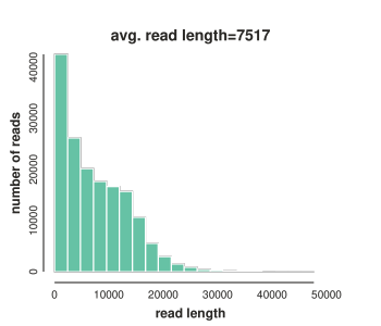
PacBio read lengths
In addition to the number of reads, we're also interested in the lengths of reads for the PacBio data, since this can vary among data sets. The commented out code below uses Python to measure the read length distribution in the PacBio data. This data is much better than the PacBio reads we looked at a few sessions ago. The average read length is around 7500bp in length (7.5kb) and many reads longer than 20kb! The commented code can produce the plot shown. Again, you do not need to run it here.
# # get lengths of each read
# with open("./SRR7825134.fastq") as indata:
#     lengths = np.array([len(next(indata)) for line in indata if line[0] == "@"])
# # plot as a barplot
# toyplot.bars(
#     np.histogram(lengths, bins=20),
#     width=350,
#     height=300,
#     xlabel="read length",
#     ylabel="number of reads",
#     label="avg. read length={:.0f}".format(np.mean(lengths))
# );
Trim reads for quality and adapters
Filtering and trimming is an important step for any genome assembly. The cleaner your reads are the better and faster the genome will assemble. The command below uses the program cutadapt to trim Illumina adapters from the reads and trim from the 3' end when quality falls below a set threshold based on the quality scores in the fastq data files. To keep our notebook easy to read we redirect the outputs normally printed to screen by cutadapt and write it to a file instead. This includes stats about how many reads were trimmed or removed. The trimming step here takes only a few minutes, but again, we've commented it out for efficiency.
We will not clean up the PacBio data files for now. These are expected to have lower quality scores, and so instead of trimming them to throw away the bad parts it is more common to try to correct the errors either as a first step before assembly, or after assembly. This can involve mapping short-read or long-reads to the long-reads before assembly, or to the assembled contigs after assembly. Pre and post-cleanup of long-read data is performed in one of the software tools we will see in the next notebook, canu.
Let's start by trimming the short read data.
# cutadapt parameters explained:
# -q: trim 3' when quality < 10
# -a: trim adapters from R1
# -A: trim adapters from R2
# -o: output R1 filename
# -p: output R2 filename
%%bash

# cutadapt \
#     -q 10 \
#     -a AGATCGGAAGAGC \
#     -A AGATCGGAAGAGC \
#     -o SRR7825135_1.trim.fastq \
#     -p SRR7825135_2.trim.fastq \
#     SRR7825135_1.fastq \
#     SRR7825135_2.fastq > trim-report.txt
The report produced by cutadapt includes statistics about how many reads were trimmed based on low quality or adapter contamination. Open the report in a new tab from this link to see the results. In the command above we named the new trimmed read files SRR7825135_1.trim.fastq and SRR7825135_2.trim.fastq. These are the files we will use going forward.
2.4% and 2.2% of read1s and reads were trimmed for adapters, respectively. The number of bases trimmed for quality scores was 81,165,611 bp (3.7%).
Genome size and complexity
Your assigned reading by Li and Harkess titled "A guide to sequence your favorite plant genomes" describes some particular difficulties of assembling plant genomes, but more broadly the advice from this paper can be generalized to many other organisms with difficult to assemble genomes as well. They make the important point that before starting any genome sequencing project it is important to learn as much as you can about your organism, as this should inform the type of approach that you take, and your expectations about the result you will get.
One of the first things you can do when you get some initial shotgun sequenced Illumina data is to investigate some of these same questions: How big is the genome, how variable, and what ploidy (has it experienced genome duplications)? It turns out we can learn answers to these questions by examining the distribution of kmer counts in the raw read data itself, without even having to map, align, or assemble it.
The second highest hump in Fig. 2B represents heterozygous sites in the genome which occur with approximately half the frequency of homozygous kmers. This can be used to estimate heterozygosity of a genome.
Jellyfish: kmer counting tool
The jellyfish program is a tool used to efficiently count kmers from a genome fasta file or fastq sequenced read files. It works much faster than the Python code we wrote last week to find all kmers in a sequence and is quite easy to use. It turns out we can learn a lot from examining the distribution of kmer counts. The quote below is from the Jellyfish paper by the authors, Marçais and Kingford (2011):
Given a string S, we are often interested in counting the number of occurrences in S of every substring of length k. These length-k substrings are called k-mers and the problem of determining the number of their occurrences is called k-mer counting. Counting the k-mers in a DNA sequence is an important step in many applications. For example, genome assemblers using the overlap-layout-consensus paradigm, such as the Celera (Miller et al., 2008; Myers et al., 2000) and Arachne (Jaffe et al., 2003) assemblers, use k-mers shared by reads as seeds to find overlaps. Statistics on the number of occurrences of each k-mer are first computed and used to filter out which k-mers are used as seeds. Such k-mer count statistics are also used to estimate the genome size: if a large fraction of k-mers occur c times, we can estimate the sequencing coverage to be approximately c and derive an estimate of the genome size from c and the total length of the reads. In addition, in most short-read assembly projects, errors are corrected in the sequencing reads to improve the quality of the final assembly. For example, Kelley et al. (2010) use k-mer frequencies to assess the likelihood that a misalignment between reads is a sequencing error or a genuine difference in sequence. A third application is the detection of repeated sequences, such as transposons, which play an important biological role. De novo repeat annotation techniques find candidate regions based on k-mer frequencies (Campagna et al., 2005; Healy et al., 2003; Kurtz et al., 2008; Lefebvre et al., 2003). The counts of k-mers are also used to seed fast multiple sequence alignment (Edgar, 2004). Finally, k-mer distributions can produce new biological insights directly. Sindi et al. (2008) used k-mers frequencies with large k (20 ≤ k ≤ 100) to study the mechanisms of sequence duplication in genomes.
Running jellyfish on the raw data files produces a .jf formatted file with information about the kmers in the data. This would take a few minutes to run. Again, we've commented it out so you can proceed to the output files.
# jellyfish parameters explained:
# -m kmer size
# -s genome size estimate
# -t number of threads to use
# -C switch to count 'canonical kmers' (reverse complement)
# -o output location
# <(...) this decompresses the file as it is passed to jellyfish
%%bash

# jellyfish count \
#     -m 21 -s 40M -t 10 -C \
#     -o 21mer.jf \
#     SRR7825135_1.fastq \
#     SRR7825135_2.fastq
After running jellyfish we can then extract a histogram from the .jf file using the histo function, which returns the histogram as a text table showing the number of unique kmers that occurred N times. You can see in the bash script above we direct the histogram to a file named 21mer.hist.csv. Again we put this file online here so that you do not have to calculate it yourself. We will load the file from this URL below to plot the kmer distribution.
%%bash

# jellyfish histo 21mer.jf > 21mer.hist.csv
Let's now use Python to load the kmer count data with the Pandas library and plot it with the Toyplot library. We can see clearly that there is a single best peak at around 55X coverage or so. We can assume that this peak represents a single copy of the genome -- all possible unique kmers in the genome have been sequenced to 55X coverage on average -- and that any other peaks represent heterozygous sites in the genome (thus the kmers at those regions only come up half as often), or errors, repetitions, and other such noise. The density of our single-copy peak stretches from about 30 to 80X.
# load the histogram data as a table
url = "https://raw.githubusercontent.com/genomics-course/11-assembly/master/notebooks/21mer.hist.csv"
df = pd.read_csv(url, sep=" ", names=["bins", "counts"])

# plot the histogram
toyplot.fill(
    df.counts[2:200],
    width=500,
    height=300,
    ylabel="number of unique kmers",
    xlabel="kmer coverage depth",
);
Genome size estimation
We can estimate the genome size by taking the total number of kmers (multiply the coverage times the number of unique kmers in each bin) and dividing this by the mean coverage (peak position). We get an estimate of ~30Mb, which is close to the current estimated value of the Bd genome of 24Mb. It's worth noting that kmer based methods for estimating genome size require high coverage of the genome, as we have here, but would not work well if our sequencing depth was much lower, say <30X.
# calculate genome size estimate
int(np.sum(df.counts[1:] * df.bins[1:]) / 55)
de novo assembly methods
There are many programs available today for genome assembly. They vary in terms of requirements of the input data, their speed, RAM requirements, and the resulting accuracy of the assemblies. For some types of data, or sizes of genomes, some tools will work better than others. Because de novo assembly is such a time consuming process it is difficult to compare many tools and so people often just use a program that others suggest. It's worth reading a few bioinformatics articles that compare assembly tools to learn more about which one might be best for your project. You were assigned an article to skim read this week by Giordano et al. in which the authors compare several assembly tools on a variety of data sets. The tool we will use below, spades, has been popular for years, and continually updated to keep pace with advancing sequencing technologies. It is a de Bruijn graph based assembly method that is best for short-read assembly, but which recently added support for hybrid assemblies that combine short-read contig assembly with scaffolding by using long-reads (HybridSpades). We will try these approaches here.
Spades
Any genome assembly software tool will include documentation about how to use it, and sometimes additional tutorials. Let's take a look at the Spades manual. In particular, take a look at the section here, titled Spades' performance. We can see when spades is applied to a test dataset of an E. coli genome (a very small genome) it takes about 8 minutes to run, uses 8.1 Gb of RAM, and uses 1.5 Gb of disk space. This is when the input data is composed of 28M reads that are 2x100bp (paired). Our data set is similar in terms of the numbers of reads, and so likely requires similar resources.
Again, we have commented out the code code below and will focus on the output files.
de novo assembly with spades: Illumina only
The command below runs a de novo assembly using Illumina data only. It first runs a pre-processing read correction step, then the main assembly of the data, and finally a post-processing contig gap filling correction step. While it is running it prints a report of its progress to the screen and to a log file. This reports what is happening in each step of the assembly, how long it has been running, and how much RAM it is consuming. Look at the log file here for this assembly.
# spades parameters explained:

# -k: if not set, then kmer size is automatically selected
# -o: output directory name
# -1: read1 inputs
# -2: read2 inputs
# -m: memory limit in Gb
# -t: number of CPU threads to use

# --only-error-correction: if set, performs read error correction only.
# --only-assembler: if set, then performs assembly only without corrections.
# --careful: if set, turns on post-processing mismatch-correction (gap filling)
# if none of these three are set then only error-correction and assembly are done by default.
%%bash

# spades.py \
#     -o assembly_spades/ \
#     -1 SRR7825135_1.trim.fastq \
#     -2 SRR7825135_2.trim.fastq \
#     -m 64 \
#     -t 20
20 threads and 64Gb of RAM were made available to the program. The read correction step took about 42 minutes. It corrected 3,033,073 bases in 2,440,874 reads. The kmer sizes used for graph assembly were 21, 33, and 55. The assembly step took 13 minutes.
Success, you just assembled a genome
Now let's try another method, by including some additional PacBio data to span the gaps between contigs in the assembly to see if we get longer scaffolds.
de novo HYBRID assembly with spades: Illumina & PacBio
To run spades in hybrid mode we can use the same command as above with just the addition of the --pacbio flag (or --nanopore if we had nanopore data) and the input fastq file for the long read data. The log file for this assembly can be found here.
%%bash

# spades.py \
#     -o assembly_spades_hybrid/ \
#     -1 SRR7825135_1.fastq \
#     -2 SRR7825135_2.fastq \
#     --pacbio SRR7825134.fastq \
#     -m 64 \
#     -t 20
Get assembly quality statistics using QUAST
The quast program is used to calculate genome quality statistics and compare assemblies. It calculates N50 contig and scaffold sizes (something we've done before), and reports BUSCO scores (number of single-copy genes present) which we've read about before. The code below will download the BUSCO single copy gene set and search for these genes in our assembled genomes. We provide it with the assembled scaffolds from both assemblies and the result will compare the two.
%%bash

# # download the busco gene set to this computer
# quast-download-busco

# # run quast to compare assemblies and find BUSCO conserved genes in both
# quast.py \
#     assembly_spades/scaffolds.fasta \
#     assembly_spades_hybrid/scaffolds.fasta \
#     -o quast_results \
#     --conserved-genes-finding \
#     --fungus
The short-read only assembly is in 1482 contigs with an N50 size of 54825 (54Kb). The hybrid assembly is in 510 contigs with an 302,379 (300Kb). The hybrid genome assembly appears to be better based on these statistics.
The two genome assemblies scored identically on (94.8%) complete BUSCO scores, and very similar on partial scores. Because these genomes are complete enough to find almost all expected single-copy genes that means they are likely pretty good assemblies and could be used for genome annotation.
Question from last time: What are PacBio 'subreads'
Subreads are the individual sequence reads that are determined in real time from a template on the sequencer. These would correspond to the stretch of DNA between the adapter sequence.
CCS reads are the result of doing a consensus base calling from subreads that are all from the same template. If the template was short enough, then the polymerase will loop entirely from the beginning back to the beginning, sequencing the adapter before it starts on the template again. In this case, the same template piece of DNA is sequenced more than once, which means that the sequence data generated from each pass can be used to determine one single consensus sequence with higher base quality than the raw subreads. Thus, the quality distribution that you see is correct between the subreads and the CCS reads