Session-10

Today's topics

1. Review notebook assignments: read lengths.

2. Discuss the assigned readings: long read technologies.

3. Introduce new topic: de Bruijn graphs.

Review of course topics

1. DNA sequencing review; and intro to Jupyter/Python.
2. Python bootcamp I: Basic objects.
3. Python bootcamp II: Scientific libraries.
4. Homology/Blast/GFF: Genome structure
5. Phylogenetics I: Sanger sequences to trees.
6. Recombination and Meiosis.
7. Inheritance and pedigrees.
8. Intro to Illumina and read mapping.
9. Intro to long-read technologies and read mapping.
10. Genome Assembly.

Notebook 9.1: Long-read sequencing

Loading fasta files as SeqIO record objects.


  # The SeqIO module is useful for working with Fasta files
  from Bio import SeqIO

  # load a Fasta file from a path with Bio
  record = SeqIO.parse(path, format="fasta")  

  # the record object makes the seq data accessible (e.g. length)
  len(record)

Notebook 9.1: Long-read sequencing

A function to load fasta files and return lengths.

   
  def getLengthDistribution(path):
      "Return a list with lengths of each fasta record"           
      lenList = []
      for record in SeqIO.parse(path, "fasta"):
          lenList.append(len(record))
      return lenList


  # example:
  getLengthDistribution("./files/sanger.aftertrim.removeCT.min500bp.fasta")


  [600, 550, 811, 430, 762, ... ]

Notebook 9.1: Long-read sequencing

A dictionary to access long file names easier.

   
  # Global dictionary of technology name to file paths.
  file_path = {
      'Sanger': 'files/sanger.total.aftertrim.removeCT.min500bp.fasta',
      'PacBio': 'files/PB.Cell1and2.raw.fasta',
      'Nanopore': 'files/LejlaControl.2D.min500bp.fasta',
  }

  # Global dictionary of technology name to colors for plotting
  colors = {
      'Sanger': '#4daf4a', 
      'PacBio': '#377eb8', 
      'Nanopore': '#984ea3',
  }

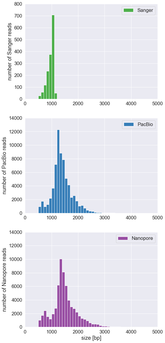
A function to plot a histogram with matplotlib.


  def makeLengthPlot(thisRunName, ax):    
      "Plot histogram of read lengths. Gets filepath from global dict"
    
      # get readlengths
      filepath = file_path[thisRunName])
      lengths = getLengthDistribution(filepath)

      # set histogram bin size
      bins = range(500, 5000, 100)

      # make histogram
      sns.distplot(
          length, bins=bins, kde=False, 
          color=colors[thisRunName], 
          ax=ax,
          label=thisRunName,
          hist_kws={"alpha": 1})

      # plot styling: legend, xlimit, ylabel, ylimit
      ax.legend()                   
      ax.set_xlim([1, 5000])        
      ax.set_ylabel('number of {} reads'.format(thisRunName))
      ax.set_ylim([0, 14000])

      # make unique y-axis label for each run
      if thisRunName == 'Sanger':
          ax.set_ylim([0, 800])

A function to plot a histogram with matplotlib.



  # initalize plot with 3 rows and 1 column
  fig, ax = plt.subplots(nrows=3, ncols=1, figsize=(8,20))

  # Plot Sanger, Pacbio, and Nanopore read length distributions
  makeLengthPlot('Sanger', ax[0]) 
  makeLengthPlot('PacBio', ax[1])
  makeLengthPlot('Nanopore', ax[2])

  # add label to x axis  
  ax[2].set_xlabel('size [bp]')

  # Show the plot
  plt.show()

Question 4 (2 points): Print the average read length and the top ten longest reads of each run.


  # 1. get filepath for Nanopore data set
  npath = file_path["Nanopore"]

  # 2. call getLengthDistribution on this file
  readlens = getLengthDistribution(npath)

  # 3. get top ten longest reads
  topten = sorted(readlens)[::-1][:10]
  print(topten)

  # 4. get average length (of all reads)
  avglen = sum(readlens) / len(readlens)
  print(avglen)


  1512.50977897917
  [298549, 108360, 72322, 67205, 61366, 60592, 45980, 45605, 41057, 39953]

Question 4 (2 points): Print the average read length and the top ten longest reads of each run.


  # get read lenghts of PacBio reads
  readlens = getLengthDistribution(file_path["PacBio"]

  # get top ten longest reads
  topten = sorted(readlens)[::-1][:10]
  print(topten)

  # get average length (of all reads)
  avglen = sum(readlens) / len(readlens)
  print(avglen)


  1370.1363583000705
  [4641, 4327, 4200, 4173, 4125, 4018, 4008, 3989, 3943, 3872]

Question 5 (1 point): What is the avg. len of PacBio reads for Susie?

12.5Kb

Notebook 9.1: Long-read sequencing

Question 6 (2 points): In Gordon et al. (2016), the authors used PacBio to assemble an entire genome, while Loomis et al. (2013) used PacBio to sequence just one gene. What is that gene and why did the authors decide to use long-read sequencing to sequence it?

The gene is Fmr1, and it is implicated in Fragile X syndrome. Fragile X is an example of a 'trinucleotide repeat disorder': healthy individuals have between 6 - 53 CGG repeats in the 5' UTR of the Fmr1 gene, while individuals with Fragile X syndrome typically have 230+ CGG repeats. Genetic analysis of these diseases have been limited by an inability to sequence regions with expanded trinucleotide repeats using short-read DNA sequencing; however, PacBio's long reads can span the length of the repetitive region to better characterize the extent of trinucleotide expansion.

Notebook 9.1: Long-read sequencing

Question 7. (3 points) Homopolymers are consecutive repetitions of a letter in a DNA sequence. For example, the sequence CATAAAG has a homopolymer of length 3, composed to the letter A. Use graph above to explain why homopolymer-length errors are common in nanopore sequencing.

There are 1024 different 5-mers but the signals typically range from about 40-70 pA: this means that normal distributions for certain 5-mers overlap, which can make it difficult to infer which 5-mer generated a particular event. If the signals for adjacent 5-mers of the DNA strand are very similar, e.g. when sequencing through long homopolymers, then the machine may not detect a change in current, which introduces sequencing error.

Oxford nanpore sequence mapping


  # read mapping always starts by "indexing" the reference fasta
  # and here also links the nanpore data.
  nanopolish index -d ecoli ecoli_2kb_region/fast5_files/ ecoli_2kb_region/reads.fasta


  [readdb] indexing ecoli_2kb_region/fast5_files/
  [readdb] num reads: 112, num reads with path to fast5: 112

Oxford nanpore sequence mapping


  # map ONT data to the reference and write output to SAM
  minimap2 -ax map-ont \
    ecoli_2kb_region/ref.fa \
    ecoli_2kb_region/reads.fasta > ecoli_2kb_region/aligned.sam


  [M::mm_idx_gen::0.289*0.60] collected minimizers
  [M::mm_idx_gen::0.318*0.80] sorted minimizers
  [M::main::0.319*0.80] loaded/built the index for 4319 target sequence(s)
  [M::mm_mapopt_update::0.333*0.81] mid_occ = 11
  [M::mm_idx_stat] kmer size: 15; skip: 10; is_hpc: 0; #seq: 4319
  [M::mm_idx_stat::0.340*0.82] distinct minimizers: 731433 (98.40% are singletons); average occurrences: 1.024; average spacing: 5.463
  [M::worker_pipeline::0.470*1.38] mapped 112 sequences
  [M::main] Version: 2.15-r915-dirty
  [M::main] CMD: ./minimap2/minimap2 -ax map-ont ecoli_2kb_region/ref.fa ecoli_2kb_region/reads.fasta
  [M::main] Real time: 0.478 sec; CPU: 0.656 sec; Peak RSS: 0.051 GB

Oxford nanpore sequence mapping

Align k-mer 'events' to the reference genome. We will run eventalign and pass in the FASTA file, the bam file, and the reference genome. The program will output the file aligned.events.txt.


  # get aligned kmer events 
  nanopolish eventalign \
    --reads ecoli_2kb_region/reads.fasta \
    --bam ecoli_2kb_region/aligned.sorted.bam \
    --genome ecoli_2kb_region/ref.fa \
    --scale-events > ecoli_2kb_region/aligned.events.txt


  [post-run summary] total reads: 537, unparseable: 0, qc fail: 0, 
  could not calibrate: 0, no alignment: 0, bad fast5: 0

Notebook 9.1: Long-read sequencing

Question 9. (3 points) Why are there four events at position 3? What happened?

The first three rows represent a scenerio in which the event detector erroneously called three events where only one should have been emitted. Note that the current for these three events are all plausibly drawn from the expected distribution `N(101.43, 1.632)`. In the fourth row, the `nanopolish` model detects that this event is a likely sequencing artefact, and therefore the output `NNNNNN` appears in the model_kmer column so that the site can be discarded before downstream analysis.

Notebook 9.1: Long-read sequencing

Question 10. (1 point) Why is the sequence of the 6-mer of the reference kmer different than the model 6-mer?

It is the reverse complement.

Notebook 9.1: Long-read sequencing

Question 11. (1 point) Each event contains a 6-mer. What is the total length of the DNA sequence that contains the set of all 6-mers represented in the `aligned_events` table?


  print(aligned_events.position.min())
  print(aligned_events.position.max())
 
  # 0
  # 4275

The first mapped position is 0, the last mapped position is 4275, the k-mer length is 6bp; thus: 1 (account for index=0) + 4275 + 6bp = 4282 bp

Principles and Applications of Modern DNA Sequencing

Session 10: de Bruijn graphs

Today's topics

Review of course topics

Notebook 9.1: Long-read sequencing

Notebook 9.1: Long-read sequencing

Notebook 9.1: Long-read sequencing

Notebook 9.1: Long-read sequencing

Notebook 9.1: Long-read sequencing

Oxford nanpore sequence mapping

Oxford nanpore sequence mapping

Oxford nanpore sequence mapping

Notebook 9.1: Long-read sequencing

Notebook 9.1: Long-read sequencing

Notebook 9.1: Long-read sequencing