Fundamentals of Evolution
EEEB G6110
Session 5: Models
Today's topics
1. Probability and Modeling in Evolution
2. Markov Models
3. Models of Molecular Evolution
4. Phylogenetic Inference
Inferring the past from the present
Statistical modeling is widely used in evolutionary research
to test or compare hypotheses and to estimate model parameters.
A model describes a mechanistic (probabilistic) process that could produce observable data. It is especially useful when
we cannot observe the past, but we can observe data at the present.
Models, Probability, and Likelihood
The use of statistical models for historical inference
is not unique to evolution, or biology, although many statistical methods were developed by biologists (e.g., the Likelihood framework was developed by the geneticist R.A. Fisher)
A likelihood function describes the probabilitiy of a set of observations given a set of model parameters.
Likelihood can express the probability of a DNA sequence alignment given a phylogenetic hypotheses, or it can express the probability that a coin toss will turn up heads versus tails.
What do we mean by a model parameter?
Models, Probability, and Likelihood
The coin toss example:
We can describe a statistical model for the outcome of a coin toss. For a single trial (a toss) there are only two possible outcomes, H or T. The probability of H is unknown. If the coin is fair then p=0.5, but maybe p!=0.5.
The probability of observing data ($D$) given model parameters ($\Theta$) is described by a likelihood function:
$$ L(\Theta) = f(D | \Theta)$$
The observed data are fixed. The function evaluates the data given proposed values for $\Theta$ and returns a score (the likelihood) for how well the parameters explain the observed data under a given model.
The goal of maximum likelihood
is to estimate $\Theta$ by finding the value that maximizes $L(\Theta)$
Models, Probability, and Likelihood
The coin toss example:
Imagine we observe the following sequence of tosses:
$$ H, T, T, H, H, H, T, T, H, H, T, T, T$$
There are multiple ways in which to describe a likelihood function based on this observation to test different hypotheses. One hypothesis we may wish to ask is whether the probability of each trial is fair (prob. heads = 0.5).
By probability theory, the outcome of many independent events is the product of their probabilities. For example, the probability of flipping heads 5 times in a row using a fair coin is:
$$ 0.5 * 0.5 * 0.5 * 0.5 * 0.5 = 0.03125 $$
Models, Probability, and Likelihood
The coin toss example:
In other words, the joint probability of multiple independent events is computed as:
$$ P(A, B) = P(A) * P(B) $$
In other words, the joint probability can be calculated as the product of many independentprobabilities:
$$ P(A_{i}) = \Pi_{i} P(A_{i}) $$
The likelihood of 5 heads in a row when p=0.5 is very low.
$$ L(\Theta=0.5) = 0.5 * 0.5 * 0.5 * 0.5 * 0.5 = 0.03125 $$
Models, Probability, and Likelihood
The coin toss example:
In other words, the joint probability of multiple independent events is computed as:
$$ P(A, B) = P(A) * P(B) $$
In other words, the joint probability can be calculated as the product of many independentprobabilities:
$$ P(A_{i}) = \Pi_{i} P(A_{i}) $$
But, the likelihood of 5 heads in a row when p=0.99 is quite high.
$$ L(\Theta=0.99) = 0.99 * 0.99 * 0.99 * 0.99 * 0.99 = 0.9509 $$
The likelihood function
The coin toss example:
The likelihood function for the probability of heads based on observed coin tosses describes the probability that a coin comes up heads (p) or tails (1-p). Since tails is just one minus heads there is only one parameter (p). The observed data is simply the number of trials (n) and the number of trials that came up heads (h):
$$ L(p) = p^{h} * (1-p)^{n-h}$$
The likelihood score depends only on the parameter (p) and the observation (n, h).
$$ L(\Theta=0.5) = (0.5)^{5} * (1-0.5)^{0}$$
$$ L(\Theta=0.99) = (0.99)^{5} * (1-0.99)^{0} $$
Statistical phylogenetics
The likelihood function calculates probability of observing a character state (DNA site in an alignment) under a specific model of molecular substitution and a phylogenetic tree (more on these soon).
Simplest models treat each DNA site independently so that the likelihood of a sequence alignment (many sites) is simply the product of the individual site likelihoods:
$$ L(D) = \prod_{i=1}^{n} L(D_{i}) = \prod_{i=1}^{n} f(D_{i} | \Theta) $$
Statistical phylogenetics
By only knowing the results of coin tosses that occurred in the past we are able to estimate the model parameters that are most likely to have produced them (i.e., the probability the coin toss is heads or tails).
The same principle applies to estimating the evolutionary distance between two aligned DNA sequences. Looking only at the results of an evolutionary process that occurred in the past we can estimate the model parameters that are most likely to have produced the DNA differences between a set of taxa.
Whereas the coin toss problem assumed a Bernoulli distribution as the underlying model, for DNA substitutions we use a molecular substitution model, which is a type of Continuous Time Markov Model.
Molecular Substitution Models
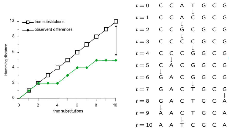
Many mutations occur that are not observable in the present-daty samples alone due to homoplasy (repeated mutations to the same sites).
Molecular Substitution Models
Instantaneous transition rate matrix ($Q$): Similar to the coin toss example, where q was equal to 1-p, you can see that the probability of not changing over some length of time is simply (1 - probability of changing.)

https://en.wikipedia.org/wiki/Models_of_DNA_evolution
Molecular Substitution Models
Transition-probability matrix: the probability of change between states over some time interval (t) is easily calculated as $ P(t) = e^{Qt} $. This tells us the probability of starting in some state (e.g., A) and ending as another (e.g., T). Jukes-Cantor Model predicts equal prob. for any state over very long branches.
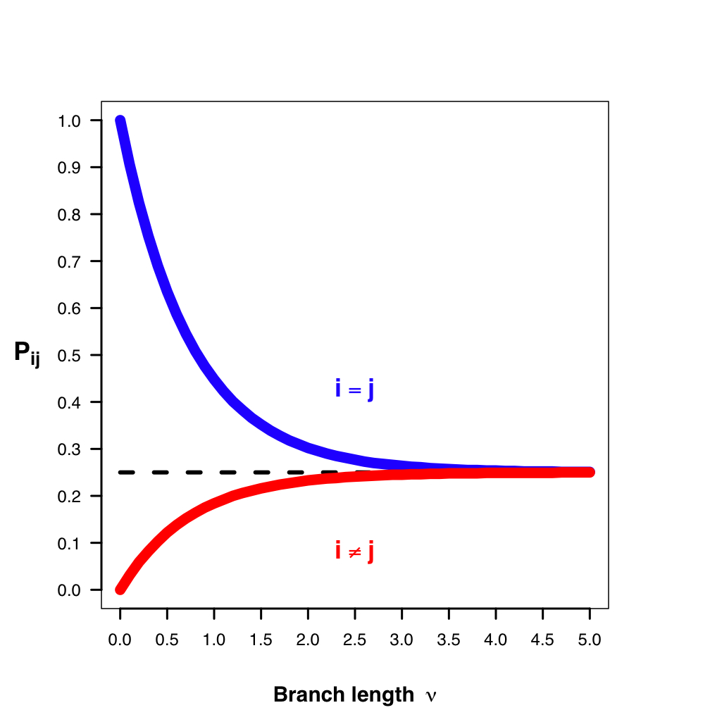
https://en.wikipedia.org/wiki/Models_of_DNA_evolution
Markov Process Models
A Markov Process is a random process in which the future state is not dependent on past states, but only on the present. (It is memory-less.)
These types of models are used extensively in evolutionary modeling, and in many other fields. Made up of a set of discrete states, starting frequencies, and a mechanism for transitioning between states.
Can be used to infer parameters (describing an unobserved process) that are most likely to produce observed data. For example, we model changes occurring in DNA sites as a Markov process.
Inferring phylogenies by ML
Felsenstein (1981) is a classic paper with >10K citations although the methods in this paper have easily been used 10-100X this often.
The likelihood of a tree is calculated as the likelihood of the data (sequence alignment) given the hypothesis (tree) under a given model (Markov substitution process).
Unlike coin tosses the likelihoods for different trees do not sum to 1. In theory, we must calculate the probabilitiy of the sequence alignment on every tree to find the maximum.
The probability of a tree hypothesis is calculated as the probability of observing substitutions along each branch of a tree. We must optimize parameters of our model (e.g., JC), and branch lengths of each tested tree.
Inferring phylogenies by ML
Felsenstein (1981) is a classic paper with >10K citations although the methods in this paper have easily been used 10-100X this often.
Felsenstein's pruning algorithm describes a simplification of the likelihood calculation that requires fewer steps by traversing a tree from tips to root and optimizing edge lengths one at a time based only on the likelihoods of the nodes descendant from each.
He describes the pulley principle as an outcome of using a reversible Markov process model ($r_{ij} = r_{ji}$). It shows that the root can be placed anywhere in the tree and does not affect the likelihood score.
Inferring phylogenies by ML
Felsenstein (1981) is a classic paper with >10K citations although the methods in this paper have easily been used 10-100X this often.
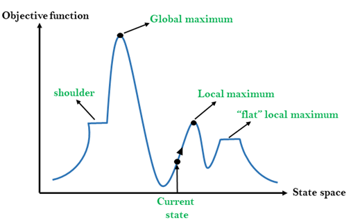
Because tree size is so large, we must use heuristic tree search algorithms to find the best tree. Felsenstein proposed a step-wise addition method to start, followed by local re-arrangements. Many similar methods are used today, involving sequential re-arrangements of the tree.
Markov Models for Evolutionary Inference
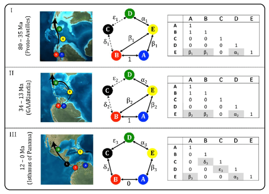
As described in your assigned review paper by O'Meara, Markov models are used widely in evolution beyond tree inference. For example, we can describe the evolution of any discrete character along branches of a tree similar to the evolution of nucleotide substitutions.
link to review of this paper.
Other common models in Evolution
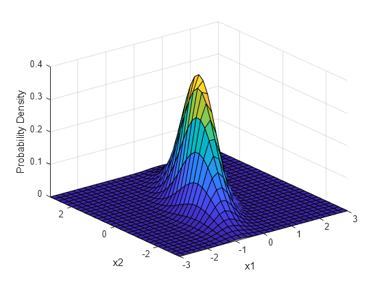
Other common classes of models used in Evolution include probability distributions (e.g., Normal), especially the Multivariate Normal Distribution, which describes covariance structure that can be used in regression framework.
Multivariate Normal Distribution describes covariance between two N distributions.
Other common models in Evolution
Phylogenetic relationships can be modeled using a variance-covariance matrix. For example, if we assume a continuous trait evolves along branches of a tree by a Brownian motion process (an assumption from the Normal Distribution) then the expeced distributions at the tips can be modeled as the sum of many independent draws from multiple normal distributions.
Multivariate Normal Distribution describes the covariance among tips of tree due to their shared ancestors (shared ancestral trait distributions).
Reading for next session
McKain Michael R., Johnson Matthew G., Uribe‐Convers Simon, Eaton Deren, and Yang Ya. 2018. “Practical Considerations for Plant Phylogenomics.” Applications in Plant Sciences 0 (0): e01038. https://doi.org/10.1002/aps3.1038.
Chapter 4 of Futuyma Textbook.