Fundamentals of Evolution
EEEB G6110
Session 8: Population Genetics II
Section topics
1. Genetic drift
2. Wright-Fisher process
3. Genealogies
4. The coalescent
5. Structured coalescent
6. Neutral theory (debate)
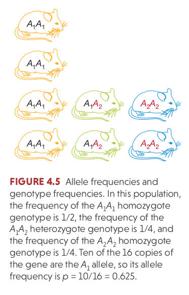
Hardy Weinberg Equilibrium
The Hardy–Weinberg principle (HW) provides the solution to one of Darwin's biggest mysteries: how variation is maintained in a population. Under Mendelian inheritance (independent assortment) the frequencies of alleles (variants at a gene) will remain constant in the absence of selection, mutation, migration, and/or genetic drift.
Binomial sampling problem
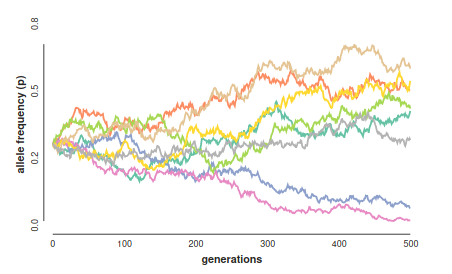
By relaxing the assumption of infinite-sized populations, this becomes a random sampling process. Diploid genotypes can be resampled each generation by sampling two alleles from the previous generation based on their frequencies. The deviations (change) in allele frequency each generation under this process is an example of genetic drift (sampling error!).
Wright-Fisher Model
By incorporating a finite effective population size (N) into our
sampling probabilities we can estimate the expected change in allele
frequencies over time (generations).
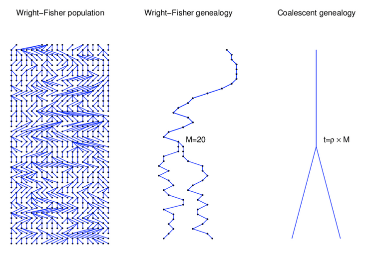
In addition to randomly sampling alleles from the previous generation, we
can *also keep track of which parental copies were passed down* (i.e., keep
track of the genealogy). This process is called the Wright-Fisher model.
A discrete time model in which each generation is composed of 2N copies of each gene. Each subsequent generation 2N new copies are randomly drawn from the previous generation.
https://en.wikipedia.org/wiki/Genetic_drift#Wright.E2.80.93Fisher_model
Wright-Fisher Model
A neutral evolutionary process (no selection) can be modeled using the WF model in which allele frequencies change over time by genetic drift.
Source: Alexei Drummond
Breaking down the Wright-Fisher Model
Genealogies are a representation of ancestor-descendant relationships. Individuals have genealogies and genes have genealogies, but their patterns are different. Whereas the number of ancestors of an individual increases in each generation back in time, the number of ancestors of a gene copy in a previous generation is always one.

Breaking down the Wright-Fisher Model
Different genes have different genealogies tracing back through different ancestors. If you continue this process back further in time, to your great-great-great-great grandparents, and so on, you will find that some of your ancestors have left no copies at any of the genes in our genome. This the basis for the concept that ones' genealogical ancestry does not match their genetic ancestry.

Breaking down the Wright-Fisher Model
Genes.
A gene (or locus) in this context refers to any non-recombined
region of the genome.
Gene copies.
A gene copy refers a single haploid copy a gene. Diploid individuals contain two copies of every gene. A gene copy in one generation may be replicated to leave many copies in the next generation.
We focus on haploids because of the assumptions of our model.
When mating is random within populations and no selection can act
on diploid genotypes, the diploid phase becomes irrelevant to our
model. A population of N diploids contains 2N gene copies.
Breaking down the Wright-Fisher Model
Coalescence: the merging of multiple gene copies into their common ancestor looking backwards in time. Because the probability that two diploid samples share a common ancestor increases rapidly backwards in time, the probability that two gene copies are descended from the same ancestral copy also increases rapidly backwards in time.

The coalescent for two gene copies
In one generation these two gene copies either came from the same parent ($ \frac{1}{2N}$)
or they came from different parents ($1 - \frac{1}{2N}$)
The probability that these two gene copies coalesced t generations ago can be calculated from these two probability statements:
$$ \left(1 - \frac{1}{2N}\right)^{t - 1} \frac{1}{2N} $$
The distribution of coalescent times
$$\mathrm{Pr}(\mathrm{coal}) = \binom{i}{2} \frac{1}{2N} = \frac{i(i-1)}{4N}$$
There are $\binom{i}{2}$ ways pairs of lineages can pick the same parent. Probability of coalescence scales quadratically with lineage count.
Expected waiting time to coalescence
$$\mathrm{E}[T_i] = \frac{4N}{i(i-1)}$$
This is a geometric distribution.
If each generation there is a $\frac{1}{x}$ probability of an event occurring, we expect to
wait $x$ generations for the event to occur.
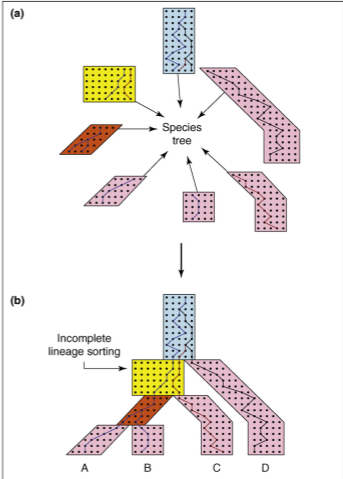
Structured (multispecies) coalescent
So far we have been working under the assumption that all samples are from a single panmictic population. But, we can also model the genealogy of sampling among multiple distinct populations.
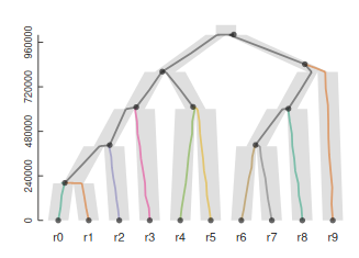
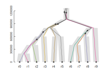
Structured (multispecies) coalescent
This can be modeled as multiple single population coalescent models combined. Starting from the tips, we ask have these n samples coalesced in this time period, if not, include them in the next chunk of model up the tree.