Fundamentals of Evolution
EEEB G6110
Session 7: Population Genetics
Section topics
1. Hardy Weinberg
2. Wright's F-statistics
3. Genealogical ancestors
4. The coalescent
5. Neutral theory (debate)
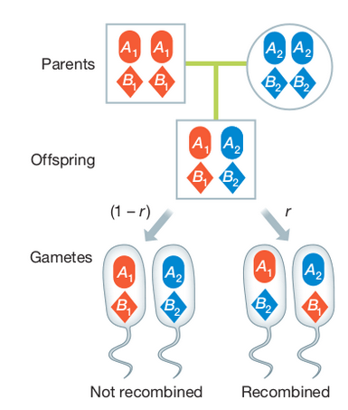
Mendelian segregation and recombination
Segregation applies to the inheritance of allele copies at a single locus, whereas recombination affects whether copies at two different loci will be inherited together.
Linkage disequilibrium
Physical linkage
Linkage describes the probability that alleles at two or more positions in the genome will be co-inherited in gametes during Meiosis. It is a measurement of an individual genome, and is influenced by the physical distance separating the alleles (the number of nucleotides in the genome), and the genetic distance (variation in recombination rates across the genome). Loci very close together tend to be in linkage disequilibrium, while those on different chromosomes tend to be in linkage equilibrium. However, selection and recombination can affect this.
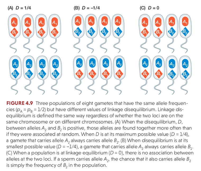
Linkage disequilibrium
Linkage disequilibrium (LD) describes the statistical association between alleles at two loci in a population, e.g., when an individual has A1 it also has B1. It is a measurement of a population and is influenced by the population history (e.g., selection, recombination), not an individual.
When a new mutation occurs the new allele only exists on the chromosome on which it evolved. It can be replicated and inherited in offspring, but will continue to occur only with the other alleles with which it is physically linked unless recombination breaks this association by crossover events that link it to other chromosomes with other alleles.
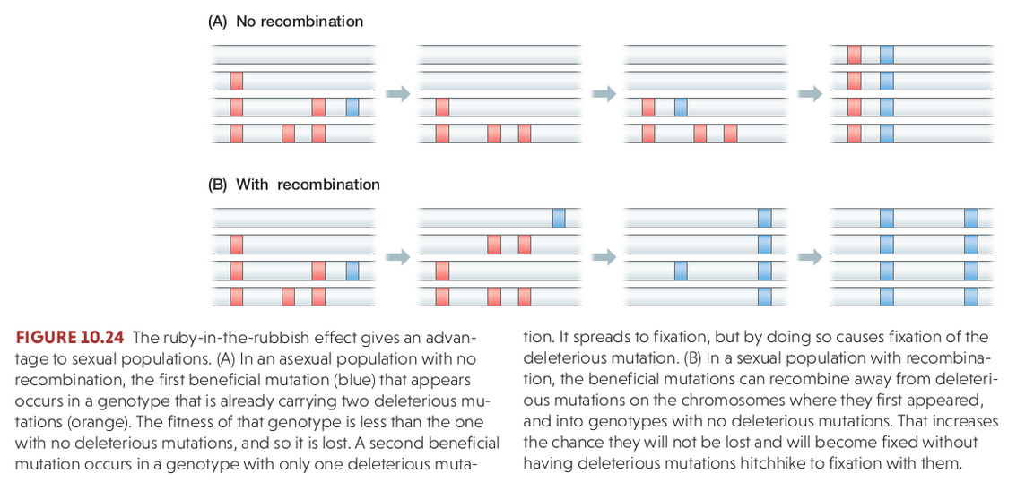
Recombination and Sex
Recombination re-shuffles variation among individuals in a population and can bring together beneficial alleles more quickly than in asexual populations.
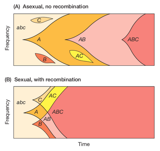
Recombination and Sex
Recombination re-shuffles variation among individuals in a population and in doing so can disassociate (linkage equilibrium) beneficial from deleterious alleles.
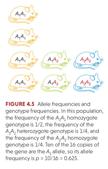
Hardy Weinberg Equilibrium
The Hardy–Weinberg principle (HW) provides the solution to one of Darwin's biggest mysteries: how variation is maintained in a population. Under Mendelian inheritance (independent assortment) the frequencies of alleles (variants at a gene) will remain constant in the absence of selection, mutation, migration, and/or genetic drift.
Hardy Weinberg Equilibrium
The Hardy–Weinberg principle (HW) provides the solution to one of Darwin's biggest mysteries: how variation is maintained in a population. Under Mendelian inheritance (independent assortment) the frequencies of alleles (variants at a gene) will remain constant in the absence of
selection, mutation, migration, and/or genetic drift.
In modeling this idealized population we make the following assumptions, and then we can also ask how allele frequencies would change if one or more of these assumptions is relaxed:
selection=0
mutation=0
migration=0 (i.e., random mating, no population structure)
Ne=infinite (infinite population size = no effect of drift)
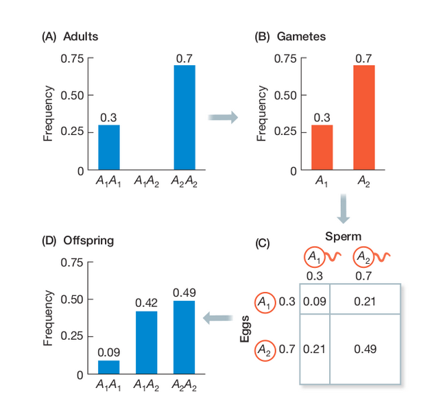
Mendelian segregation and recombination
In the absence of evolutionary processes causing allele frequency changes, the frequency of diploid genotypes in a population will change only according to the probability of mating (random sampling).
At any single locus the two copies can be passed on with equal probability (segregation) and so Hardy-Weinberg equilibrium can be reached within a single generation:
$p^{2} + 2pq + q^{2} = 1$.
Hardy Weinberg Equilibrium
The three genotypes for a locus with two alleles will occur at: $p^{2} + 2pq + q^{2} = 1$.
Wright-Fisher Model
By incorporating a finite effective population size (N) into our sampling probabilities we can estimate the expected change in allele frequencies over time (generations).
A discrete time model in which each generation is composed of 2N copies of each gene. Each subsequent generation 2N new copies are randomly drawn from the previous generation. The probability of obtaining k copies the next generation is:
$$ {{2N \choose k}p^{k}(1-p)^{2N-k}} $$
https://en.wikipedia.org/wiki/Genetic_drift#Wright.E2.80.93Fisher_model
Wright-Fisher Model
A neutral evolutionary process (no selection) can be modeled using the WF model in which allele frequencies change over time by genetic drift.
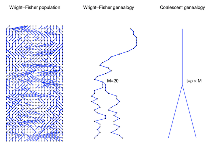
Source: Alexei Drummond
Wright-Fisher Model
In addition to estimating the effects of genetic drift on allele frequencies in a single population, Sewall Wright developed a series of estimators for predicting how differences between populations could evolve by genetic drift.
Wright's F-statistics (fixation indices) describe these probabilities in terms of sampling probabilities (i.e., bean-bag genetics).
A central measurement of F-statistics is the inbreeding coefficient (F).
$$ F = 1 - \frac{Observed(Aa)}{Expected(Aa)} $$
Wright's F-statistics
Under HW the genotype frequencies in a populations are:
$$ AA = p^{2} $$
$$ Aa = 2pq $$
$$ aa = q^{2} $$
In the presence of inbreeding (non-random mating)
these deviate from HW as:
$$ AA = p^{2}(1-F) + pF $$
$$ Aa = 2pq(1 - F) $$
$$ aa = q^{2}(1-F) + qF $$
Wright's F-statistics
These statistics become interesting when we start to define what we mean by a population. For example, comparing sampled individuals from two locations.
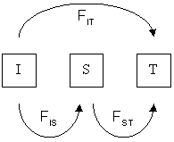
Different F-statistics look at different levels of population structure. $F_{IT}$ is the inbreeding coefficient ($F$) of an individual relative to the total population. $F_{IS}$ is the inbreeding coefficient of an individual relative to a subpopulation ($S$), and $F_{ST}$ is the effect of subpopulations relative to total.
Wright's F-statistics
$F_{ST}$ can be interpreted as a measure of population differentiation. If $F_{ST}$ between two populations is 1 then they are fixed for different alleles (no variation is segregating in both populations).
Wright's F-statistics
For example, large populations among which there is much migration tend to show little differentiation, whereas small populations among which there is little migration tend to be highly differentiated. FST is a convenient measure of this differentiation, and as a result FST and related statistics are among the most widely used descriptive statistics in population and evolutionary genetics.
$F_{ST}$ applied
The most widely used of these statistics is $F_{ST}$, as we are often interested in the effect of population subdivision, and in comparing genetic diversity of subpopulations. There are several definitions of $F_{ST}$:
$$ F_{ST} = \frac{\pi_{between}-\pi_{within}}{\pi_{between}} $$
Or, the variance in p across populations over the max variance that could exist among subpopulations.)
$$ F_{ST} = \frac{var(p)}{p(1-p)} $$
$F_{ST}$ applied
The most widely used estimator of $F_{ST}$ from DNA sequence data is:
$$ F_{ST} = \frac{\pi_{between}-\pi_{within}}{\pi_{between}} $$
Where $\pi_{between}$ and $\pi_{within}$ are the average number of pairwise differences between two individuals sampled from different subpopulations (between) or the same subpop (within). This estimator is also biased and so we typically use another estimator, Watterson's $\Theta$, to estimate the average pairwise distance as population genetic diversity (more on this next time).
$F_{ST}$ in humans
Genetic diversity in humans is low compared to our close relatives, and most variation is shared among human populations.
Based on three million SNPs, ~12% of the genetic variation is found to occur between continental populations, and ~1% between populations within continents.
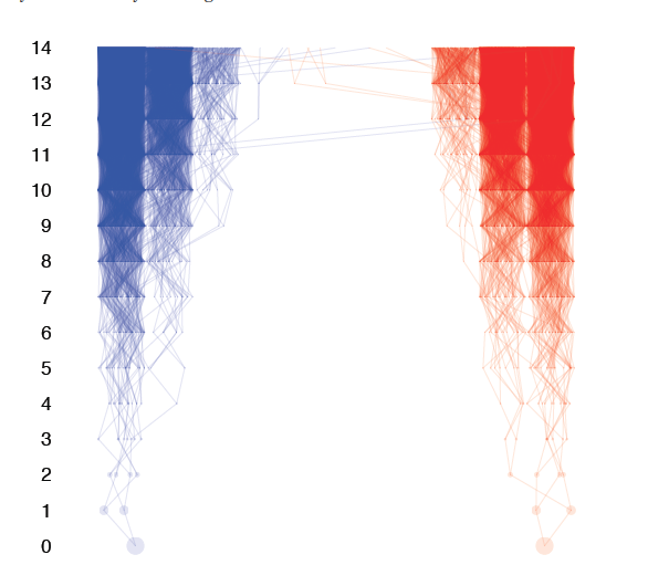
Wright-Fisher Model
A neutral evolutionary process (no selection) can be modeled using the WF model in which allele frequencies change over time by genetic drift.
Source: Alexei Drummond
Genealogical ancestors
The number of ancestors doubles every generation. The time backwards until n samples share a common genealogical ancestor is surprisingly small.
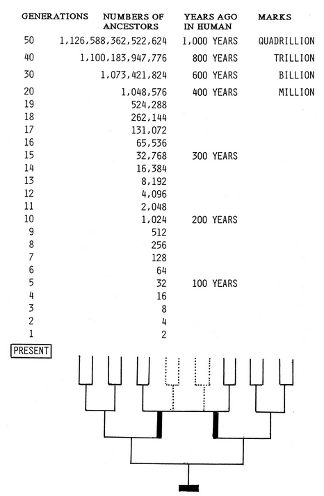
Genealogical ancestors
This is true even among samples that include people from distant geographic regions. Some of their ancestors may have dispersed further and because each population has so many ancestors, some are likely to be shared.
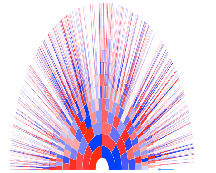
Genealogical ancestors
Each genealogical ancestor does not contribute equally to an individuals genome. In fact, *very few* genealogical ancestors are highly represented genetically. Most of your ancestors leave no genetic trace in your genome.
The neutral theory of molecular evolution
Neutral theory proposes that most genetic variation within species and genetic differences among species are a result of genetic drift acting on selectively neutral alleles.
Most new mutations are deleterious and lost, or weakly deleterious and thus effectively neutral. Beneficial mutations are rare and fix quickly and thus will not be observed as within-population variation.
A recent neutral theory debate
"The Neutral Theory in Light of Natural Selection." (Kern and Hahn, 2018).
"The importance of the Neutral Theory in 1968 and 50 years on: A response to Kern and Hahn 2018." (Jensen et al. 2018).
Summarize the arguments from both sides. Form an opinion.