Isolation, interference, and introgression: genomic perspectives on plant diversification
Deren Eaton
Dept. of Ecology, Evolution, and Environmental Biology
Columbia University
How can we most accurately reconstruct the
evolutionary history
of organisms from their genomes?
How can genomics (i.e., evolutionary inference)
be used to reconstruct historical
ecological interactions among species?
Phylogenomic sampling
Characterize evolutionary history from a subset of sampled genomes (individuals).


Phylogenomic sampling
Characterize whole genomes from a subset of sequenced markers.

Genealogical variation
It is important to examine evolutionary history across the entire genome.

Historical introgression/admixture
Introgression is common throughout the history of many lineages.

Historical introgression/admixture
But there are many potential sources of error in these analyses...
Genealogical variation

How can we most accurately reconstruct the
evolutionary history
of organisms from their genomes?
Software development

Phylogenomic inference methods

Missing data in RAD-seq and other methods

Missing data in RAD-seq and other methods

ipyrad-analysis toolkit
Filter or impute missing data; easily distribute massively parallel jobs.
  import ipyrad.analysis as ipa

  # initiate an analysis tool with arguments
  tool = ipa.pca(data=data, ...)

  # run job (distribute in parallel)
  tool.run()

  # examine results
  ...
ipyrad-analysis toolkit
Filter or impute missing data; easily distribute massively parallel jobs.
  tool = ipa.pca(data=data, imap=imap, minmap=minmap, mincov=0.5)
  tool.run(nreplicates=20, seed=123)
  tool.draw(2, 3);

Window_extracter: extract, filter, format.
Reference mapped RAD loci can be "spatially binned" to form larger loci.
  import ipyrad.analysis as ipa

  # initiate an analysis tool with arguments
  tool = ipa.window_extacter(
      data=data,
      scaffold_idx=0,
      start=0,
      end=1000000,
  )

  # writes a phylip file
  tool.run()
Window_extracter: extract, filter, format.
Reference mapped RAD loci can be "spatially binned" to form larger loci.

Window_extracter: extract, filter, format.
Reference mapped RAD loci can be "spatially binned" to form larger loci.

Herbicide resistance among Amaranthus species.

Phylogenomic methods: gene trees

Gene tree inference
Faces two distinct problems:
(1) individual loci (e.g., RAD tags) are often insufficiently informative;
(2) most "loci" do not contain a single gene tree.

Gene tree inference
Faces two distinct problems:
(1) individual loci (e.g., RAD tags) are often insufficiently informative;
(2) most "loci" do not contain a single gene tree (even short RAD tags).
Gene tree inference
We have a recent preprint on this topic: phylogenetic half-life
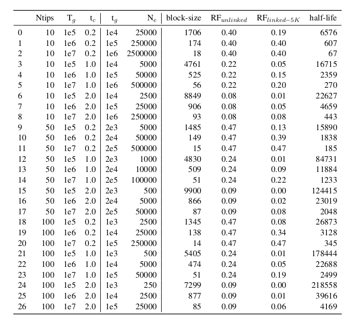
ipcoal: simulate genealogies and loci in spp. trees
At any reasonable phylogenetic scale the size of non-recombined loci is small!
  import ipcoal

  # simulate data with demographic parameters
  model = ipcoal.Model(tree=newick, Ne=5e5, mut=1e-8, recomb=1e-9)

  # simulate n loci of a given length
  model.sim_loci(nloci=1, nsites=500)

Decaying Phylogenomic methods: SNPs

Phylogenomic methods: SNPs
The Phylogenetic invariants framework
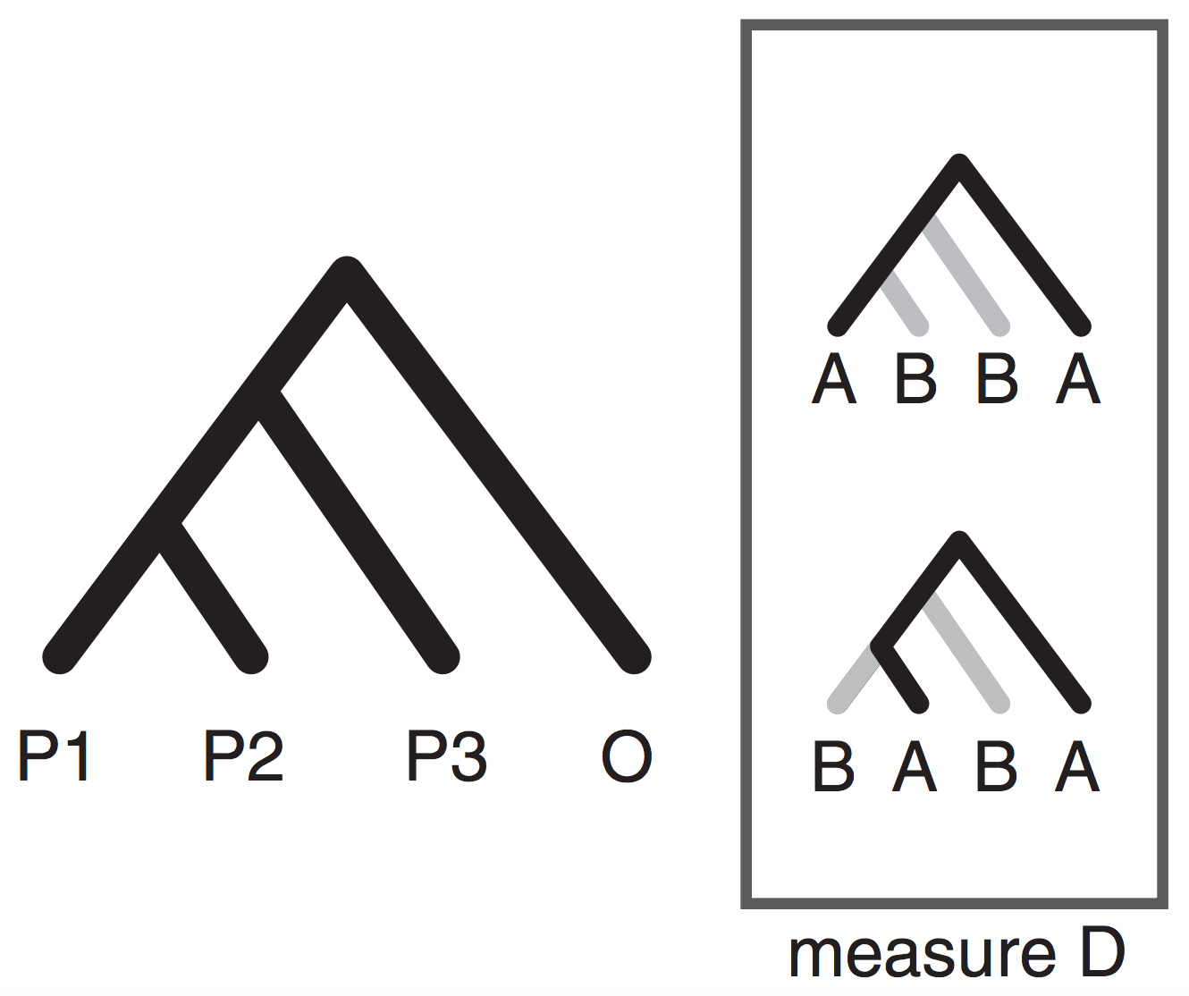
Phylogenetic invariants are SNP patterns that are expected to occur in equal proportions given the existence of a split/edge on a tree (e.g., AAGG = GGAA). Some invariant patterns have been of particular interest as a metric for quantifying admixture (e.g., BABA, ABBA).
Identifying invariant patterns for a tree can be difficult, but is easy for small trees. Most invariant methods focus on 4-taxon trees.
The SVDquartets species tree inference method organizes SNP patterns into a matrix where algebraic symmetries make it easy to identify the correct unrooted topology for any four taxa.


SVDquartets reduces SNP matrices to categorical results

SVDquartets reduces SNP matrices to categorical results

SVDquartets reduces SNP matrices to categorical results

Shortcoming of the SVDquartets approach
By reducing the quantative SNP frequency data to a categorical relevant information for inferring admixture is lost (e.g., ABBA-BABA; Durand et al. 2011).
Moving beyond ABBA-BABA
Higher level invariants (e.g., 5-taxon patterns) also exist and can provide even more information about admixture (Eaton et al. 2012, 2015). A difficult part of applying 4 or 5-taxon tests to larger tree, however, is that summarizing the results of many non-independent tests has not been automated and becomes difficult.
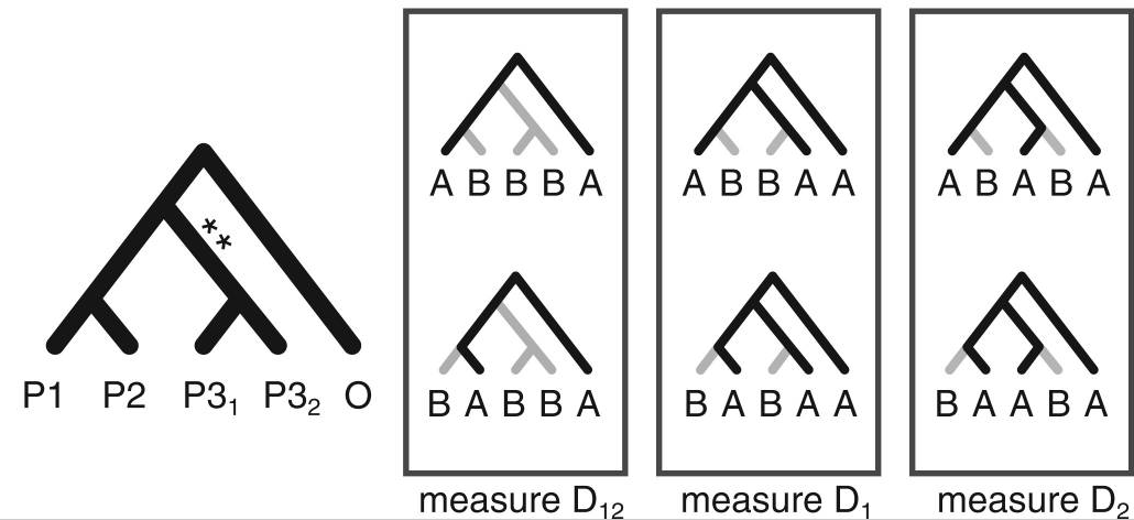
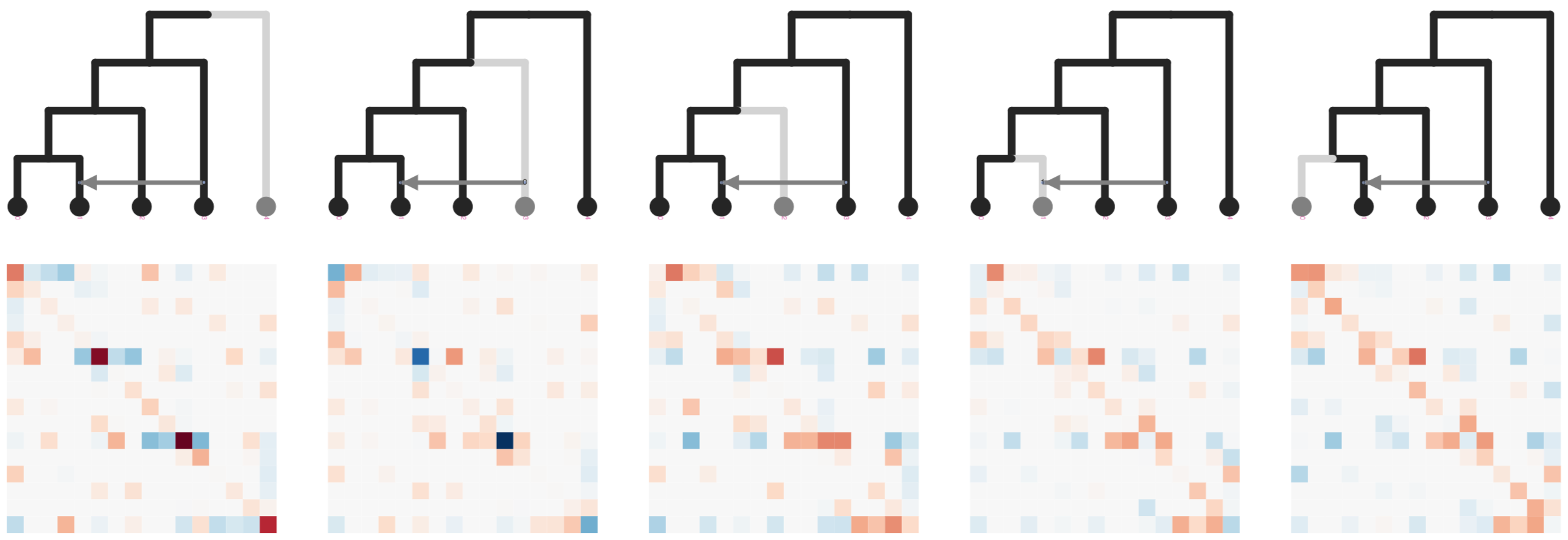
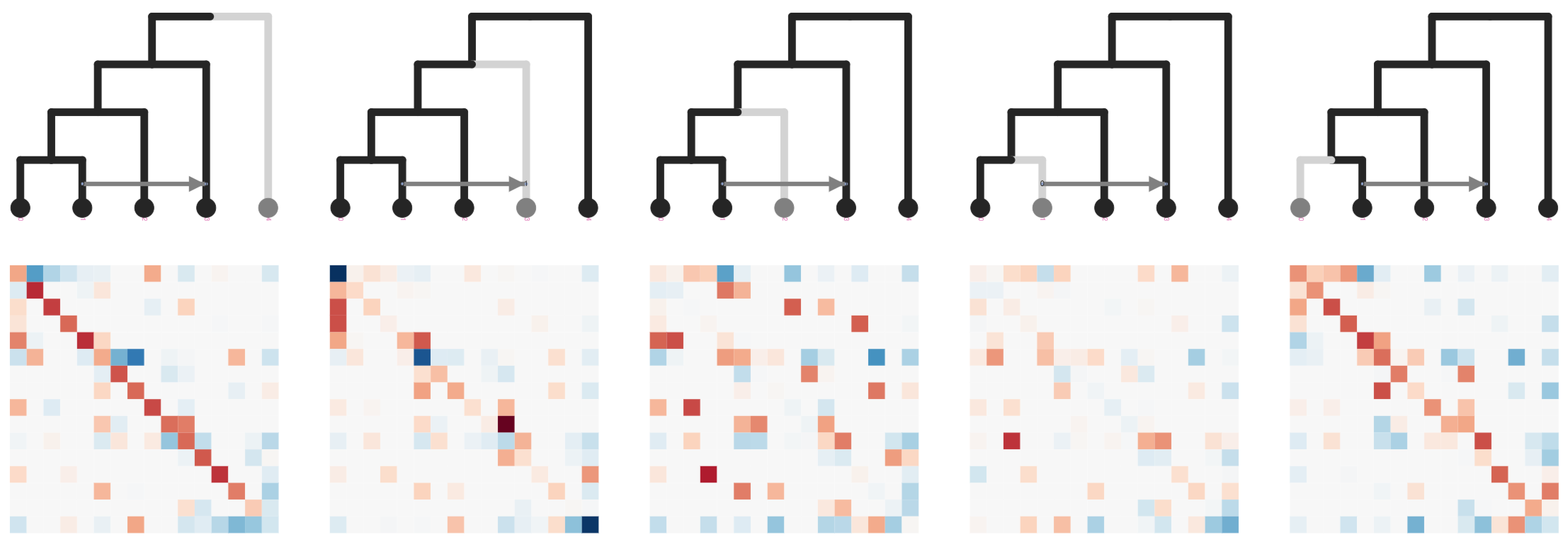
Stacked matrices for inferring admixture edges
Stacked matrices for inferring admixture edges
Stacked matrices for inferring admixture edges
Stacked matrices for inferring admixture edges

Stacked matrices for inferring admixture edges

Stacked count matrices
Unique fingerprint for different admixture scenarios
simcat: inference of admixture edges from machine
learning on phylogenetic invariants
ExtraTrees Classifier (scikit-learn) is trained on simulated SNP count data and invariant features extracted from stacked matrices: ABBA-BABA (Durand et al. 2011); Hils statistics (Kubatko and Chifman 2019).
User inputs a species tree estimate to simcat, and it tests all admixture edge placements, and simulates over variable edge lengths, and demographic parameters.

Patrick McKenzie
Eaton lab PhD student
Simulation and training a neural network on SNPs from network topologies

simcat: machine learning on phylogenetic invariants
The classifier is able to infer the correct placement of admixture
edges at >95% accuracy with only 20K SNPs and <1 day of training for smallish trees (<= 8 taxa).
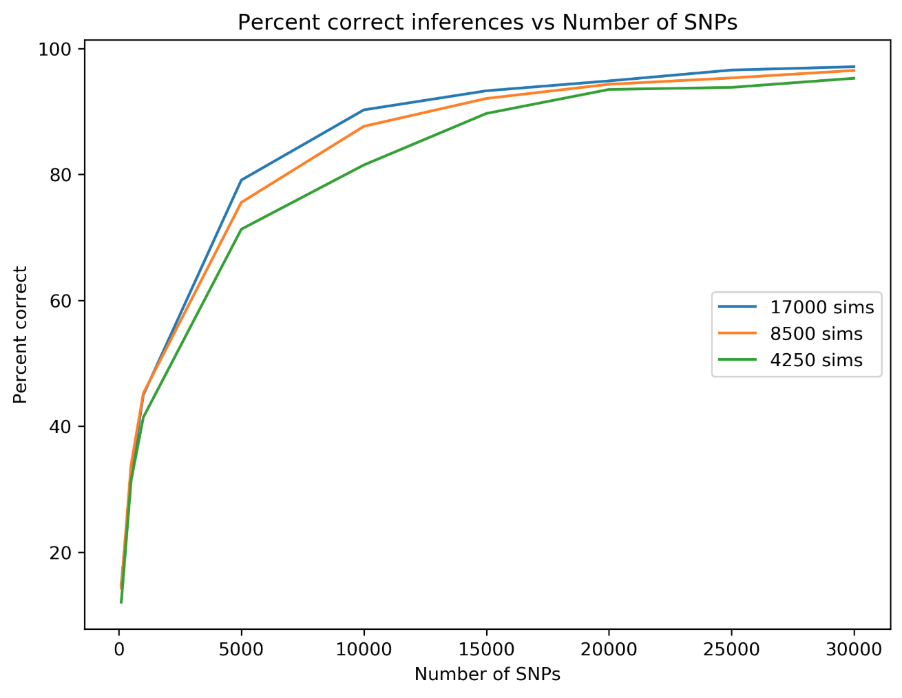
The strengths of this approach are both practical and theoretical
In practice: SNPs are easier to obtain than informative gene trees. And millions of SNPs may be able to detect more subtle patterns than hundreds of genes.
In theory:, informative gene trees do not exist for distantly related taxa (concat-alescence). And, phylogenetic invariants assume a general Markov Model that does not require optimizing parameters (even branch lengths!). It is a topology test.
Coming soon: Software tool for application to empirical data.
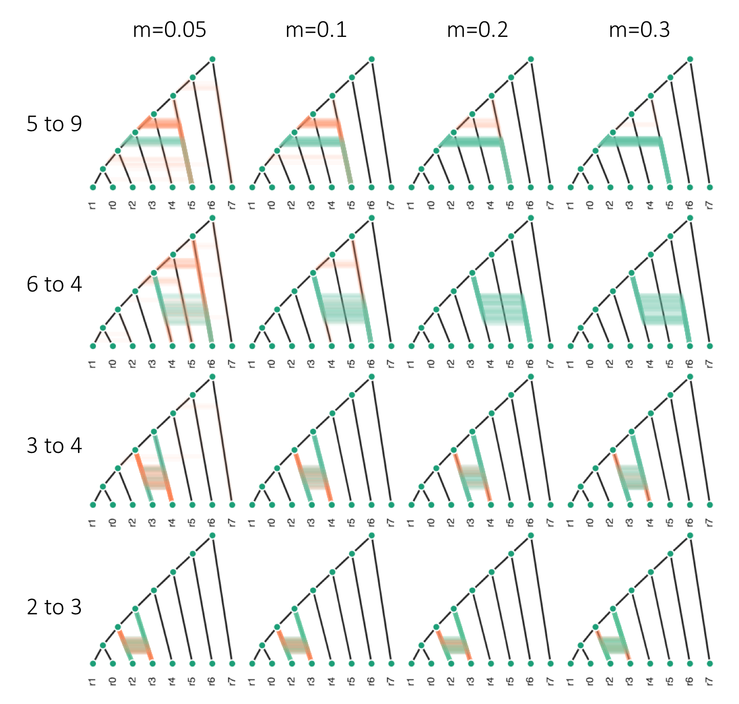
High accuracy despite huge demographic variance. Simcat trains on topologies!
How can we use genomics to reconstruct historical
ecological interactions among species?
The Hengduan Mountains
The Hengduan Mountains
The Hengduan Mountains
The Hengduan Mountains
The Hengduan Mountains
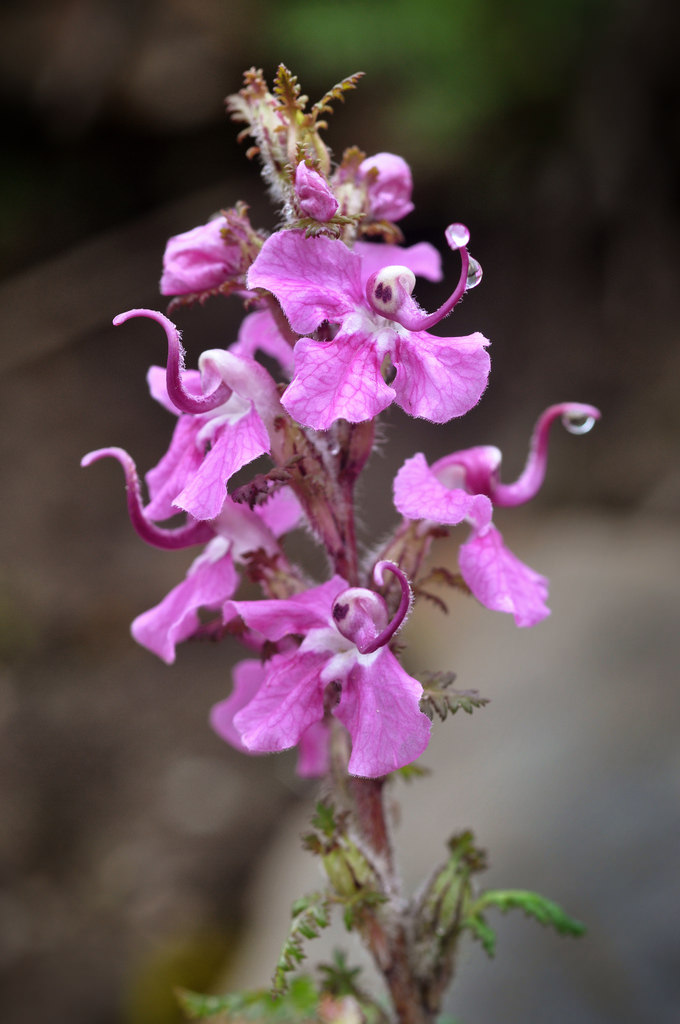
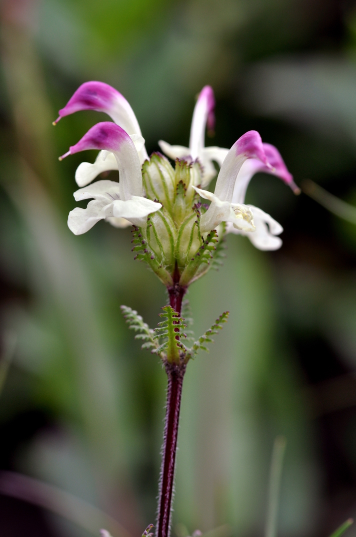
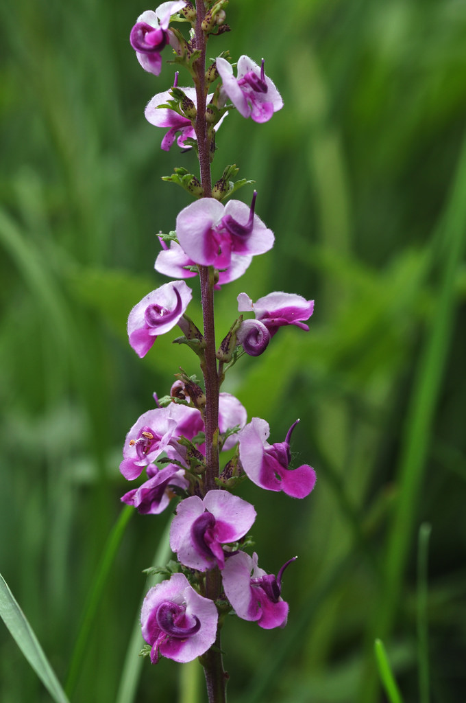
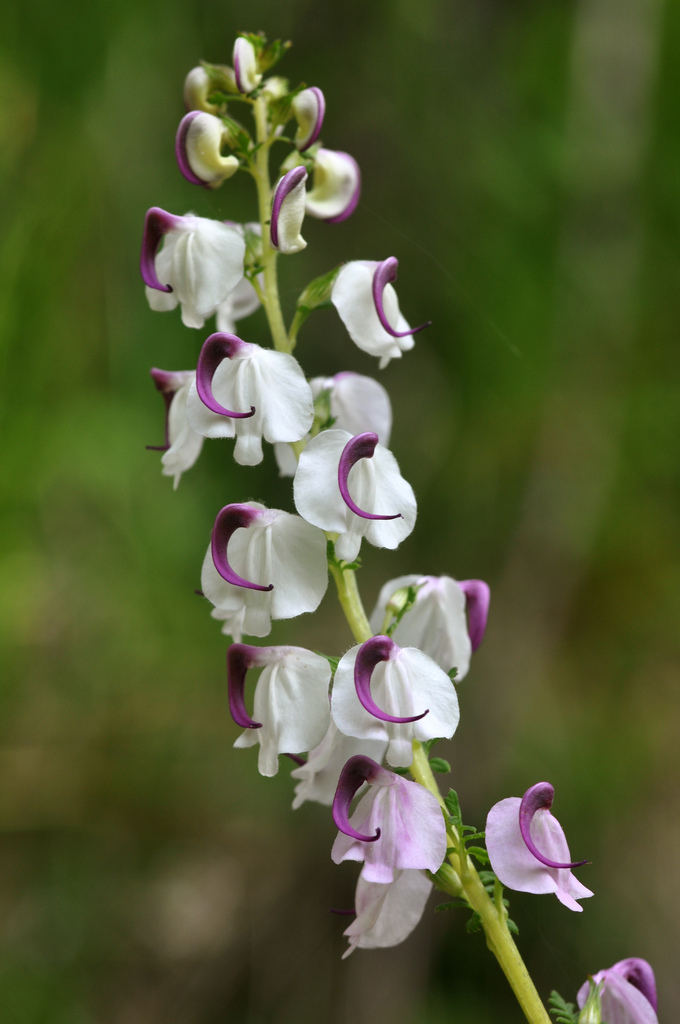
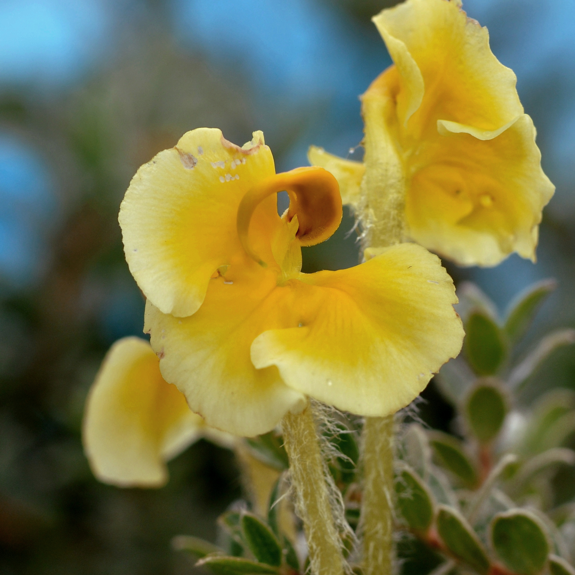
Floral diversity in Pedicularis


Pedicularis L. in China
Species rich:
>600 species worldwide, approximately 300 endemic to Hengduan.
We collected >100 species (>2100 specimens) from >300 locations in 2018-2019.
Morphologically diverse:
Spectacular floral diversity and abundant homoplasy;
similar forms have evolved repeatedly (Ree 2005)
Complex history of assembly:
Mountain uplift over millions of years, glacial cycles over
thousands of years, river and mountains barriers, lead to
constantly shuffling communities (and species
interactions).
Reproductive interference
Negative fitness consequences imposed by one organism on another by disrupting successful reproduction.

Ecological pattern: reproductive interference
Phenotypic overdispersion (limiting similarity) and
phylogenetic
randomness (homoplasy)
in assembly of Pedicularis species into communities (Eaton & Ree 2012).

Evolutionary process: character displacement
Divergent selection drives greater differences between populuations in sympatry than allopatry (e.g., benthic/limnetic sticklebacks) to reduce competition for limited resources.

Evolutionary process: character displacement
The difficulty for Pedicularis is that there are so many species that each interacts with: who is the focal competitor? We need a community model of character displacement.

Does interspecific competition/interference drive floral divergence?
Is floral divergence associated with genetic divergence/speciation?
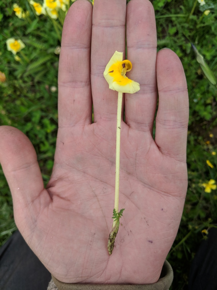
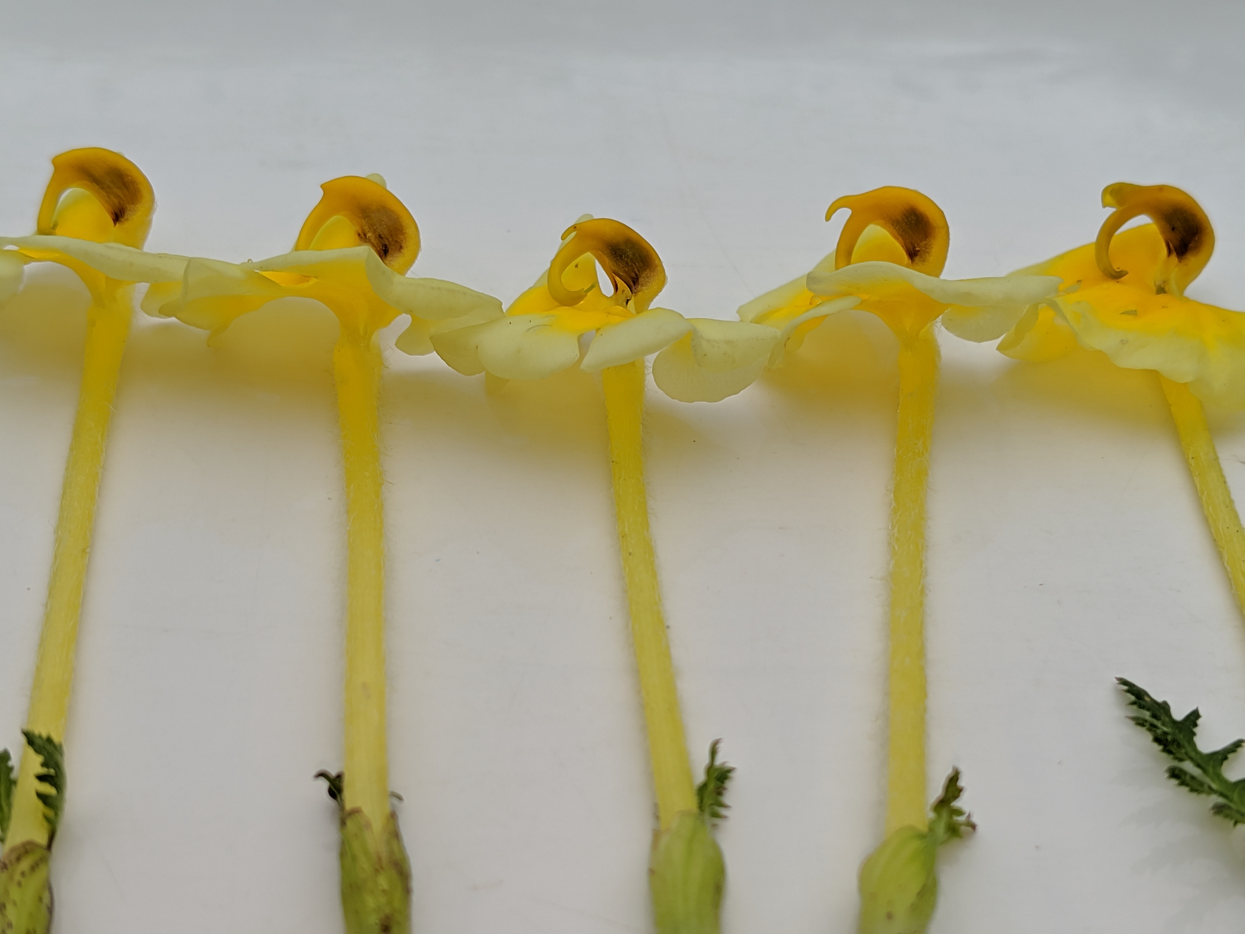
Morphological terminology

The beak of the galea directs pollen placement and pickup

Elongate styles
Elongate styles have evolved multiple times (Ree 2005) and facilitate pollen competition among species (Tong and Huang 2016).


Reproductive character displacement
Hypothesis: Differences among populations (within species) are a result of interspecific interactions driving character displacement in local communities.

Case study: Pedicularis cranolopha

Case study: Pedicularis cranolopha

P. cranolopha
P. longiflora
P. rhinanthoides

P. fetisowii
Testing association between phenotype and (biotic) environment

P. cranolopha RAD-seq genomics
110 individuals from 15 targeted locations.
RAD-seq (original) PstI enzyme, ~5M reads per sample;
ipyrad min50 assembly: 20K loci, 21% missing, 286K SNPs

P. cranolopha RAD-seq genomics

P. cranolopha RAD-seq genomics

P. cranolopha RAD-seq genomics
Style length does not correlate strongly with genetic clades.

P. cranolopha RAD-seq genomics
Migration estimates are highly asymmetic (migrate-n; 100 loci): the southern-most clade (Yunnan) is a sink of gene flow. Very different relation from tree-based inference.

Testing association between phenotype and (biotic) environment
Lande (1976):
Selection pulls
the mean phenotype towards a local optimum, while
Gene Flow homogenizes phenotypes among populations,
and they evolve by stochastic
Drift.


Felsenstein (2002):
Eigen decomposition of the known migration matrix
yields a transformation to get independent trait means
(no covariances) and expected variances.
Model summary: breaking it down
1. Focal phenotype (style length) measure across 15 populations.
2. Migration matrix estimated from
RAD data to model expected covariation of focal phenotypes.
3. Local biotic variables
phenotypic and phylogenetic distance to other Pedicularis in
each community. We will model local optima as a function of these
measurable variables.
Implementation: Bayesian hierarchical regression model in pyMC3: Fit residuals between observed and transformed trait means with biotic variables (allowing different slopes for different species).
A community phylogenetic test for character displacement
The phylogenetic model is a poor fit to the data whereas the phenotypic nearest neighbor distance model fits well. Posterior distribution of model parameters:

P. cranolopha has a longer style when co-occurring with closer relatives; supports gametophytic "arms-race" hypothesis.
Experiment: Does style length variation affect gene flow?

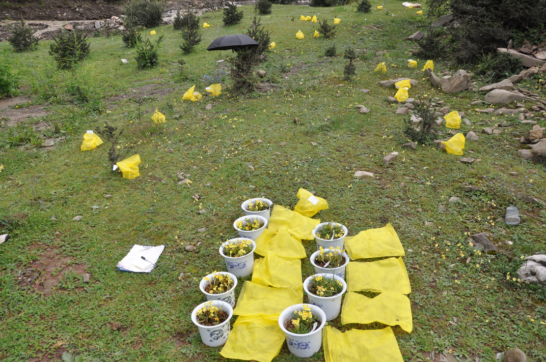
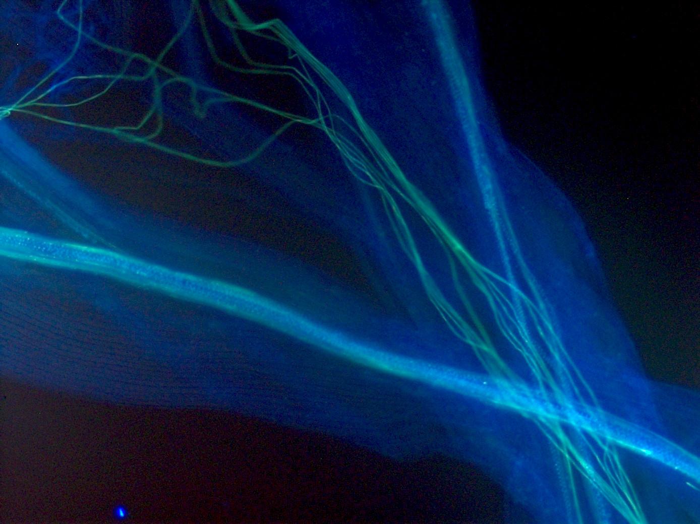
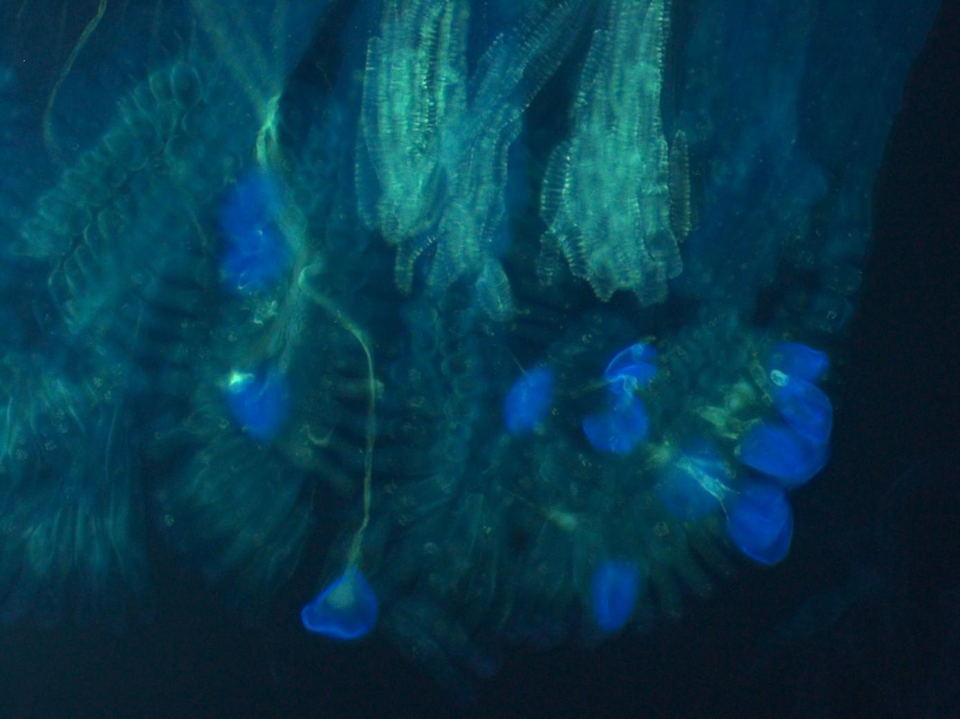

Larger pollen grows faster and further, consistent with 10X higher migration from long to short style populations inferred from genomic data.
Systematics of the P. cranolopha complex
Taxonomically challenging; split into species/subspecies based on style length, pubescence, and presence of a "forked beak".


Pollen transfer occurs on the right side of bumblebee pollinators
but is not highly precise, bees tend to squirm about.
In forked populations bees are restrained in the "fork", which may increase precision.
Systematics of the P. cranolopha complex
Hybrid zones: contact between populations with "forked beak" and without.
Systematics of the P. cranolopha complex
Hybrid zones: contact between populations with "forked beak" and without.
1
2
2
3
Horned beak variation within hybrid zone 1.
Summary
The ipyrad-analysis toolkit makes it easy to deal
with missing data, file formats, replication, and reproducibility.
SNP-based tree and network inference methods are the future. While genealogies are real, informative gene trees are not (except plastids).
In Pedicularis species interactions drive reproductive character
displacement which likely accelerates floral evolution and diversification.
Acknowledgements
Richard Ree
Dave Boufford
Huang Shuang-Quan
De-Zhu Li
Patrick McKenzie
Jared Meek
Kasi Molina-Velez
Sandra Hoffberg
Isaac Overcast
NSF DEB
NSF DDIG
NSF EAPSI
Columbia Lenfest Award